Preprocessing of Optically Pumped Magnetometer (OPM) data

Introduction

Optically Pumped Magnetometers (OPMs) are magnetic field sensors that can be used for MEG as an alternative to the conventional SQUID sensors. SQUIDs are superconductive sensors that require cryocooling, and hence need to be placed as an array in a fixed helmet-shaped dewar that is filled with extremely cold liquid helium.

OPMs are individual sensors that do not need a dewar for the cryocooling. Due to their small size, OPMs are more flexible in their placement and allow for other recording strategies. For example, you can use a small number of OPMs (or even one) and do sequential recordings in which you position then over different places over the scalp.

An important difference between OPMs and most SQUID-based MEG systems is that OPMs are magnetometers, whereas most conventional MEG systems consist of (mostly) gradiometers. Gradiometers are designed to suppress the environmental field, as explained in this video. Magnetometers see more of the environmental noise and consequently the static earth magnetic field can also become visible as noise due to (small) movements. Movements of the head, and thereby of the sensors, cause the OPMs to move through the residual earth magnetic field in the MSR. As head movements are relatively slow, this results in low-frequency noise.

This tutorial focusses on preprocessing of OPM data and some simple analyses. Following the computation of the ERFs, you could you could in principle continue with source reconstruction: the early components of the median nerve lend themselves well to dipole fitting. However, since no coregistration was performed between the head and sensors, it is not possible to construct an accurate headmodel or to plot the sources on top of the anatomical MRI of the participant.

Most follow-up analyses are not specific to OPMs and are demonstrated in other tutorials. Detecting and dealing with large movements and suppressing environmental noise in the OPM magnetometers, for example using homogenous field compensation (HFC) with ft_denoise_hfc, will also not be covered in this tutorial.

Background

In this tutorial we will use recordings made with a small set of 8 OPM sensors during somatosensory stimulation of the median nerve. The OPM sensors were placed over three different configurations over the region of interest and the experimental stimulation protocol was repeated three times. This results in ERFs over 24 different locations over the head. The combined topography of these ERFs can be plotted. This requires that we rename each channel to make it consistent with the location in the helmet where it was recorded, and appending the three separate recordings in one.

The participant was seated in a magnetically shielded room that also houses a Neuromag SQUID-based MEG system. Note that the Neuromag system is without a cryocooler; this is relevant as the cryocooler cold head would have introduced additional noise.

The dataset used in this tutorial

OPM recordings were done using a FieldLine v2 system comprised of 8 OPMs sensitive in the radial (or axial) direction. The OPMs were placed in a FieldLine alpha-1 helmet, which allows them to be slide inwards, touching the scalp surface.

The participant received electrical stimulation of the median nerve of the right hand. We therefore expect an N20 component over the left somatosensory cortex. The median nerve stimulation protocol was repeated three times, with different positions of the OPM sensors. An Excel sheet was used to document the mapping of which sensor (or channel) was placed where.

The data for this tutorial can be downloaded here from our download server.

Procedure

In this tutorial we will take the following steps:

• Initial look at the data using ft_databrowser
• Define trials and read the data using ft_preprocessing
• Renaming the channels using a montage
• Removing artifacts using ft_rejectvisual and ft_badsegment
• Compute the averaged ERFs using ft_timelockanalysis
• Concatenate the data over the three positions using ft_appendtimelock
• Improve the whole-head ERF topoplot using ft_prepare_layout
• Plotting the OPM sensor positions in 3D using ft_plot_sens

Initial look at the data

We start with a quick initial look at the data in ft_databrowser. This allows us to check the signals but also some extra information such as how many channels the data contains, the channel labels, and how triggers are encoded.

cfg = [];
cfg.dataset = 'MedianNerve_StimBreakStim2min_Pos1.fif';
cfg.ploteventlabels = 'no';
cfg.preproc.demean = 'yes';
cfg.ylim = [-1 1]*1e-11;
ft_databrowser(cfg)

Another way to get information about the data in the file is by reading the header using the low-level ft_read_header function.

hdr = ft_read_header('MedianNerve_StimBreakStim2min_Pos1.fif');

This shows that we have 9 channels (8 for the OPMs and one for the triggers), that the sampling rate is 1000Hz, that the recording is about 6 minutes (365120 samples divided by 1000 is 365 seconds) and some other details.

 hdr =
   struct with fields:

           label: {9x1 cell}
          nChans: 9
              Fs: 1000
            grad: [1x1 struct]
        nSamples: 365120
     nSamplesPre: 0
         nTrials: 1
            orig: [1x1 struct]
        chantype: {9x1 cell}
        chanunit: {9x1 cell}

We can do the same for the events with the low-level ft_read_event function:

event = ft_read_event('MedianNerve_StimBreakStim2min_Pos1.fif');

There are 733 events corresponding to the electrical stimulation of the median nerve. The first event reveals that the type is Input-1 and the value is 1; this is relevant for defining the trials or segments of interest.

 event(1)
 ans =
   struct with fields:

         type: 'Input-1'
       sample: 130
        value: 1
       offset: []
     duration: []

Define trials and read the data

Using ft_definetrial we proceed to define the segments of interest. This will again read the events and determine a segment around each of them.

cfg = [];
cfg.trialdef.eventtype = 'Input-1';
cfg.trialdef.prestim = 0.1;
cfg.trialdef.poststim = 0.3;

cfg.dataset = 'MedianNerve_StimBreakStim2min_Pos1.fif';
cfg = ft_definetrial(cfg);

The field cfg.trl represents the trials or segments of interest. We proceed by reading the data corresponding to the trials:

cfg.channel = '00*';
cfg.detrend = 'yes';
cfg.baselinewindow = [-inf 0];
data_pos1 = ft_preprocessing(cfg);

cfg = [];
cfg.lpfilter = 'yes';
cfg.lpfreq = 0.5;
cfg.channel = '00*';
cfg.dataset = 'MedianNerve_StimBreakStim2min_Pos1.fif';
data_pos1_continuous = ft_preprocessing(cfg);

cfg = [];
cfg.dataset = 'MedianNerve_StimBreakStim2min_Pos1.fif';
cfg.trialdef.eventtype = 'Input-1';
cfg.trialdef.prestim = 0.1;
cfg.trialdef.poststim = 0.3;
cfg = ft_definetrial(cfg);

% the trl field defines the trials
trl = cfg.trl;

% cut the trials from the continuous data in memory
cfg = [];
cfg.trl = trl;
data_pos1_segmented = ft_redefinetrial(cfg, data_pos1_continuous)

Just like the first recording, we read the recordings that were done with the OPM sensors in the 2nd and 3rd position:

cfg = [];
cfg.trialdef.eventtype = 'Input-1';
cfg.trialdef.prestim = 0.1;
cfg.trialdef.poststim = 0.3;

cfg.dataset = 'MedianNerve_StimBreakStim2min_Pos2.fif';
cfg = ft_definetrial(cfg);

cfg.channel = '00*';
cfg.detrend = 'yes';
cfg.baselinewindow = [-inf 0];
data_pos2 = ft_preprocessing(cfg);

cfg = [];
cfg.trialdef.eventtype = 'Input-1';
cfg.trialdef.prestim = 0.1;
cfg.trialdef.poststim = 0.3;

cfg.dataset = 'MedianNerve_StimBreakStim2min_Pos3.fif';
cfg = ft_definetrial(cfg);

cfg.channel = '00*';
cfg.detrend = 'yes';
cfg.baselinewindow = [-inf 0];
data_pos3 = ft_preprocessing(cfg);

Renaming the channels

Each OPM sensor has a serial number. Furthermore, each sensor is connected to a channel in the electronics chassis. The serial numbers are not starting from 1, but the electronics channels are. However, we don’t care which sensor is attached to channel “1”, we care where each channel is relative to the head.

The FieldLine alpha-1 helmet has 107 slots in which the sensors can be placed. Each of the slots has a name, like “FLxx”, and during the recording an excel sheet was used to keep track of which channel was connected to which sensor, and in which slot each sensor was placed. We use that information to rename the channels. We can use a montage for that, combined with ft_apply_montage. A montage is usually used to implement a more complex re-referencing scheme, such as bipolar channels in intracranial EEG (see this example), but can also be used for simple renaming of the channels.

chassis = {1   2   3   4   5  6   7  8};
sensor  = {338 119 323 111 62 336 22 246};
pos1 = {'FL30'   'FL21' 'FL20' 'FL23' 'FL36' 'FL35' 'FL34' 'FL84'};
pos2 = {'FL30_2' 'FL38' 'FL37' 'FL28' 'FL27' 'FL19' 'FL18' 'FL84_2'};
pos3 = {'FL30_3' 'FL22' 'FL29' 'FL39' 'FL45' 'FL44' 'FL43' 'FL84_3'};

montage_pos1 = [];
montage_pos1.labelold = {
  '00:01-BZ_OL'
  '00:02-BZ_OL'
  '00:03-BZ_OL'
  '00:04-BZ_OL'
  '00:05-BZ_OL'
  '00:06-BZ_OL'
  '00:07-BZ_OL'
  '00:08-BZ_OL'
  }';
montage_pos1.labelnew = pos1; % labels according to the helmet
montage_pos1.tra = eye(8);

The montage_pos1.tra field is an identity matrix, which means that each channel is simply copied over from the original data to the new data. The only difference is in the old and new channel names.

montage_pos2 = [];
montage_pos2.labelold = {
  '00:01-BZ_OL'
  '00:02-BZ_OL'
  '00:03-BZ_OL'
  '00:04-BZ_OL'
  '00:05-BZ_OL'
  '00:06-BZ_OL'
  '00:07-BZ_OL'
  '00:08-BZ_OL'
  }';
montage_pos2.labelnew = pos2; % labels according to the helmet
montage_pos2.tra = eye(8);

montage_pos3 = [];
montage_pos3.labelold = {
  '00:01-BZ_OL'
  '00:02-BZ_OL'
  '00:03-BZ_OL'
  '00:04-BZ_OL'
  '00:05-BZ_OL'
  '00:06-BZ_OL'
  '00:07-BZ_OL'
  '00:08-BZ_OL'
  }';
montage_pos3.labelnew = pos3; % labels according to the helmet
montage_pos3.tra = eye(8);

Now that we have the three montages, we can use the cfg.montage option in ft_preprocessing, or directly call the low-level ft_apply_montage function.

cfg = [];
cfg.montage = montage_pos1;
data_pos1 = ft_preprocessing(cfg, data_pos1);

cfg.montage = montage_pos2;
data_pos2 = ft_preprocessing(cfg, data_pos2);

cfg.montage = montage_pos3;
data_pos3 = ft_preprocessing(cfg, data_pos3);

Exercise 1

Removing artifacts

As the OPM sensors are magnetometers, there will be some noise that they pick up. With the small number of channels in each of the recordings, denoising is not so easily done. We have a lot of trials and we can remove those that show a lot of noise.

The summary method in ft_rejectvisual offers a quick screening of the whole data and allows to select trials that are to be rejected.

cfg = [];
cfg.method = 'summary';
data_pos1_clean = ft_rejectvisual(cfg, data_pos1);

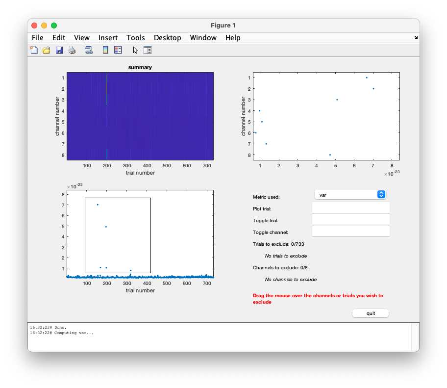
When you look at the maximum variance in each of the trials (the subplot in the lower left), a variance threshold of 2e-24 appears appropriate to remove the more noisy ones.

We use the same method for the data at the other two positions:

data_pos2_clean = ft_rejectvisual(cfg, data_pos2);
data_pos3_clean = ft_rejectvisual(cfg, data_pos3);

The variance threshold that we identified was 2e-24, which is in units of Tesla-squared. We can also use the standard deviation as the metric, which is the square root of the variance. That gives sqrt(2e-24) corresponding to a threshold of 1.4e-12 (or 1.4 pT).

With ft_rejectvisual we manually click in the figure to select the threshold. If we know the threshold that we want to apply and we want to make it consistent over all recordings, we can also use the ft_badsegment function. That function does not reject the trials immediately, like ft_rejectvisual, but merely marks where the artifacts are, just like most other artifact detection functions. This is explained in more detail in the introduction on dealing with artifacts. The ft_rejectartifact function does the actual work in removing them from the raw data structures.

cfg = [];
cfg.metric = 'std';
cfg.threshold = 1.4e-12;
[cfg, artifact] = ft_badsegment(cfg, data_pos1);

data_pos1_clean = ft_rejectartifact(cfg, data_pos1);

cfg = [];
cfg.metric = 'std';
cfg.threshold = 1.4e-12;
[cfg, artifact] = ft_badsegment(cfg, data_pos2);

data_pos2_clean = ft_rejectartifact(cfg, data_pos2);

cfg = [];
cfg.metric = 'std';
cfg.threshold = 1.4e-12;
[cfg, artifact] = ft_badsegment(cfg, data_pos3);

data_pos3_clean = ft_rejectartifact(cfg, data_pos3);

Do note that the trials are 400ms long with 100ms baseline, and that the stimuli are only ~300ms spaced. Consequently the trials are partially overlapping and the number of artifacts detected and number of trials removed does not match: there are artifacts that are present in multiple consecutive trials.

Exercise 2

cfg.artifact.badsegment.artifact = artifact;

Compute the averaged ERFs

Now that we only have the clean trials left, we can average them to obtain the ERF.

cfg = [];
timelock_pos1 = ft_timelockanalysis(cfg, data_pos1_clean);
timelock_pos2 = ft_timelockanalysis(cfg, data_pos2_clean);
timelock_pos3 = ft_timelockanalysis(cfg, data_pos3_clean);

Concatenate the data over the three positions

The three data structures with the ERFs for the 3x8 positions can be concatenated using the ft_appendtimelock function.

cfg = [];
cfg.appenddim = 'chan';
timelock = ft_appendtimelock(cfg, timelock_pos1, timelock_pos2, timelock_pos3);

% FIXME I am not sure why this is needed
timelock.avg = timelock.trial;
timelock = rmfield(timelock, 'trial');

The resulting data structure contains 24 channels.

Visualize the ERFs

We can visualize the ERFs from the OPM data just as we would do with other MEG or EEG data, as explained in the plotting tutorial](/tutorial/plotting). For that we need a layout which specifies the location of each channel in the figure. The construction of a layout is explained in the layout tutorial; but in this case we can use the template layout that is included in FieldTrip.

cfg = [];
cfg.layout = 'fieldlinealpha1_helmet.mat';
cfg.showlabels = 'yes';
cfg.ylim = 'maxabs';
ft_multiplotER(cfg, timelock);

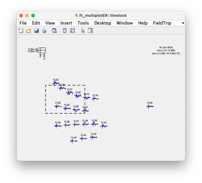
The multiplot figure is interactive and you can click in the figure to make a selection of channels.

Subsequently, you can click again to make a selection over time to get to a topographic figure.

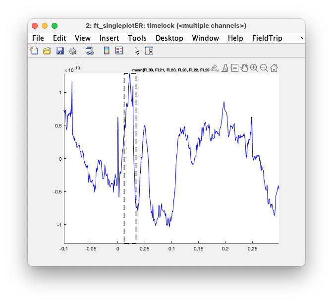
Exercise 3

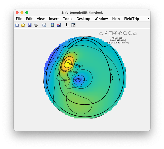
We can make the same topographic figure by calling ft_topoplotER.

cfg = [];
cfg.layout = 'fieldlinealpha1_helmet.mat';
cfg.marker = 'labels';
cfg.xlim = [0.019 0.028];
cfg.zlim = 'maxabs';
ft_topoplotER(cfg, timelock);

You should notice that the topographic interpolation of the data spans the whole head, whereas we only recorded recorded the activity over the left somatosensory cortex (and one channel on the right). That means that most of the field distribution that you see cannot be trusted, as it is extrapolated.

Interpolating (and extrapolating) is exactly what ft_topoplotER is supposed to do, as it needs to assign a color code to each location around the head, also to those locations where no sensor was placed.

Improve the visualization of the ERFs

The ft_multiplotER function determines the intersection between the data and the layout and only shows those channels. We know that there are many more slots in the helmet and showing those can help to interpret the spatial distribution. We can achieve this by “padding” the ERF data with NaN or Not-a-Number values.

We fist identify the channels in the layout that are not present in the measurement:

load fieldlinealpha1_helmet.mat  % this contains the layout
missing = setdiff(layout.label, timelock.label);
missing = missing(startsWith(missing, 'FL'));

We can then make a copy of the ERF and add the channels

% make a copy of the original timelock structure, remove two fields that we don't care about
timelock_full = rmfield(timelock, {'dof', 'var'});

% add the extra slots from the helmet that are missing in the recording
timelock_full.label = cat(1, timelock_full.label(:), missing(:));
timelock_full.avg   = cat(1, timelock_full.avg, nan(numel(missing), numel(timelock_full.time)));

Prior to adding the channels that were not recorded, we had the following labels:

 timelock.label'
 ans =
   1x24 cell array
   Columns 1 through 10
     {'FL30'}    {'FL21'}    {'FL20'}    {'FL23'}    {'FL36'}    {'FL35'}    {'FL34'}    {'FL84'}    {'FL30_2'}    {'FL38'}
   Columns 11 through 20
     {'FL37'}    {'FL28'}    {'FL27'}    {'FL19'}    {'FL18'}    {'FL84_2'}    {'FL30_3'}    {'FL22'}    {'FL29'}    {'FL39'}
   Columns 21 through 24
     {'FL45'}    {'FL44'}    {'FL43'}    {'FL84_3'}

After adding the fake channels with NaN values, we get a full ERF structure that looks like this:

 timelock_full.label'
 ans =
   1x111 cell array
   Columns 1 through 10
     {'FL30'}    {'FL21'}    {'FL20'}    {'FL23'}    {'FL36'}    {'FL35'}    {'FL34'}    {'FL84'}    {'FL30_2'}    {'FL38'}
   Columns 11 through 20
     {'FL37'}    {'FL28'}    {'FL27'}    {'FL19'}    {'FL18'}    {'FL84_2'}    {'FL30_3'}    {'FL22'}    {'FL29'}    {'FL39'}
   Columns 21 through 30
     {'FL45'}    {'FL44'}    {'FL43'}    {'FL84_3'}    {'FL1'}    {'FL10'}    {'FL100'}    {'FL101'}    {'FL102'}    {'FL103'}
   Columns 31 through 40
     {'FL104'}    {'FL105'}    {'FL106'}    {'FL107'}    {'FL11'}    {'FL12'}    {'FL13'}    {'FL14'}    {'FL15'}    {'FL16'}
   Columns 41 through 50
   ...

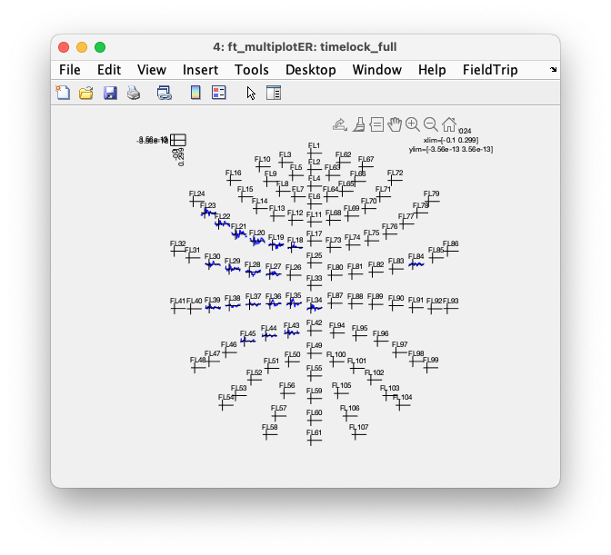
We can again plot it, and you’ll see that the fake channels are now displayed. Of course they don’t show any data, but at least you can see where they are.

cfg = [];
cfg.layout = 'fieldlinealpha1_helmet.mat';
cfg.showlabels = 'yes';
cfg.ylim = 'maxabs';
ft_multiplotER(cfg, timelock_full);

If you now use the mouse to make a selection over a few channels, and then make a selection over the N20 latency range (or use the following code), you again get a topographic plot.

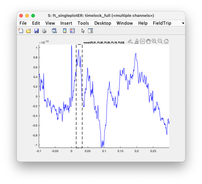
You’ll get the same plot with the following code.

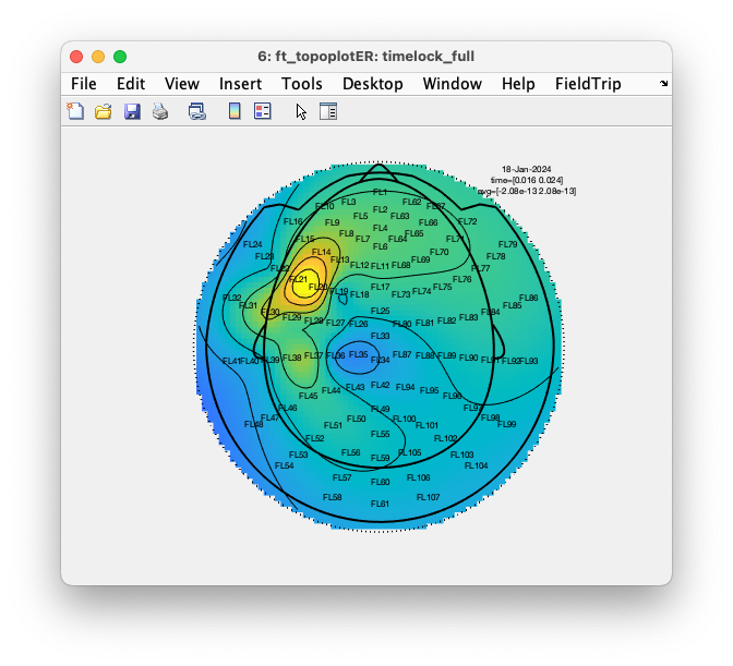
cfg = [];
cfg.layout = 'fieldlinealpha1_helmet.mat';
cfg.marker = 'labels';
cfg.xlim = [0.016 0.024];
cfg.zlim = 'maxabs';
ft_topoplotER(cfg, timelock_full);

Note how this figure is even more deceiving than the previous one, as the interpolation of the colors is still over the whole head, but it now also shows dots at the location of all channels, including the ones where we inserted NaNs as fake data. This makes it look as if there was actually a measurement at those locations.

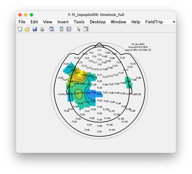
Since the fake channels contain NaNs, we are now able to tell the function to exclude those from the interpolation using the cfg.interpolatenan option. By default that is set to ‘yes’, but here we want to set it to ‘no’.

cfg = [];
cfg.layout = 'fieldlinealpha1_helmet.mat';
cfg.marker = 'labels';
cfg.xlim = [0.016 0.024];
cfg.zlim = 'maxabs';
cfg.interpolatenan = 'no';
ft_topoplotER(cfg, timelock_full);

The result is an topographic interpolation where the fake channels are shown as dots, but where the NaN value has not been replaced by an interpolated/extrapolated color.

Mask the topographic interpolation

Adding fake channels with NaNs to the data and using the cfg.interpolatenan option is one way to make a topography that shows the whole head without incorrect colors over areas where we did not record. Another way is described here; this is based on a modified version of the layout.

We start with loading the layout

cfg = [];
cfg.layout = 'fieldlinealpha1_helmet.mat';
cfg.skipcomnt = 'no';
cfg.skipscale = 'no';
layout = ft_prepare_layout(cfg);

or

load fieldlinealpha1_helmet.mat  % this contains the layout

To avoid confusion, let’s rename the layout structure in memory into layout_full.

layout_full = layout
clear layout

We can check that it consists of 107 channels, plus a location for the “Comment” and a location for the “Scale”.

 layout_full
 layout_full =
   struct with fields:

         pos: [109x2 double]
       label: {109x1 cell}
       width: [109x1 double]
      height: [109x1 double]
     outline: {1x5 cell}
        mask: {[101x2 double]}
         cfg: [1x1 struct]

Besides the 107 channel labels and the two for the Comment and Scale, their locations, their width and their height, there is also a field for the outline (i.e., the head-shaped circle with two ears and a nose) and a field for the mask. The mask determines the spatial extent of the interpolation, so usually it is identical to the head-shaped circle in the outline.

We can make another version of the layout with a reduced number of channels. If we discard the mask field, it can be recreated based on a convex hull around the channels that are remaining.

cfg = [];
cfg.layout = rmfield(layout_full, 'mask');
cfg.channel = timelock.label;
cfg.mask = 'convex';
layout_trimmed = ft_prepare_layout(cfg);

The trimmed layout now contains 22 channels; also the mask contains fewer line segments (now 13, which was 101).

 layout_trimmed
 layout_trimmed =
   struct with fields:

     pos: [22x2 double]
   label: {22x1 cell}
   width: [22x1 double]
  height: [22x1 double]
 outline: {1x5 cell}
     cfg: [1x1 struct]
    mask: {[13x2 double]}

Using the trimmed mask we can again make the topoplot of the ERF.

cfg = [];
cfg.layout = layout_trimmed;
cfg.marker = 'labels';
cfg.xlim = [0.016 0.024];
cfg.zlim = 'maxabs';
ft_topoplotER(cfg, timelock);

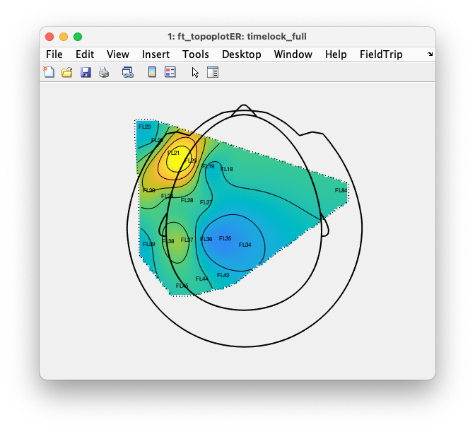
It is not ideal yet, as there are mostly channels over the left somatosensory cortex but also one channel ‘FL84’ on the right, which remain connected by the interpolation.

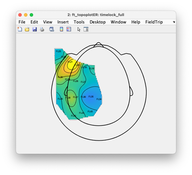
An even better trimmed layout can be constructed if we also exclude channel ‘FL84’:

cfg = [];
cfg.layout = rmfield(layout_full, 'mask');
cfg.channel = setdiff(timelock.label, 'FL84');
cfg.mask = 'convex';
layout_trimmed = ft_prepare_layout(cfg);

cfg = [];
cfg.layout = layout_trimmed;
cfg.marker = 'labels';
cfg.xlim = [0.016 0.024];
cfg.zlim = 'maxabs';
ft_topoplotER(cfg, timelock);

Plotting the OPM positions in 3D

The multiplot and the topoplot are both projections on the 2D surface of our screen. It can be helpful to look at the OPM sensors in 3D. For that we can load the full definition of the sensors.

close all
load fieldlinealpha1 % this contains the fieldlinealpha1 structure, similar to the grad structure in the data

figure
ft_plot_sens(fieldlinealpha1, 'label', 'yes', 'axes', 1, 'orientation', 1, 'chantype', 'megmag', 'fiducial', 1)

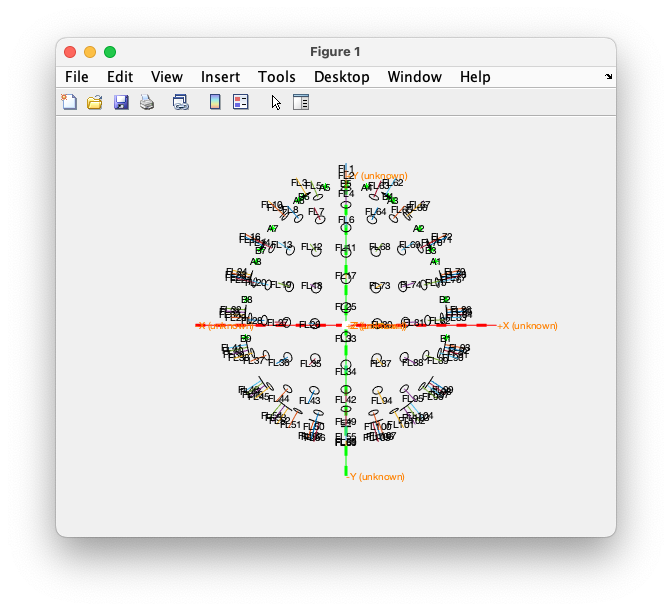
You can rotate this 3D figure by using the Rotate 3D option in the upper right corner of the figure and by dragging it with your mouse.

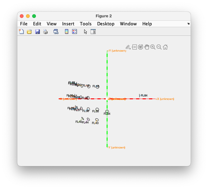
Again it makes sense to look at the specific selection of OPM sensors that was used in the recordings.

fieldlinealpha1.chantype( ismember(fieldlinealpha1.label, missing)) = {'missing'};
fieldlinealpha1.chantype(~ismember(fieldlinealpha1.label, missing)) = {'megmag'};

figure
ft_plot_sens(fieldlinealpha1, 'label', 'yes', 'axes', 1, 'orientation', 1, 'chantype', 'megmag', 'fiducial', 0)

Summary and suggested further reading

This tutorial gave an introduction on processing OPM data, specifically dealing with a small OPM array that was used to record activity sequentially over multiple locations that together cover the region-of-interest. Furthermore, it showed how to plot the data topographically, given that not the whole head was covered by the measurement.

You may want to continue with the more general tutorials on processing MEG (and EEG) data, or have a look at the system specific details for the OPM data that you are working with. Also, you could have a look at the tutorial about coregistration of OPM data.

Furthermore, you can explore example scripts that deal with OPMs:

and frequently asked questions:

• Getting started with Cerca OPM data
• Coregistration of Optically Pumped Magnetometer (OPM) data
• Getting started with FieldLine OPM data
• Template 2-D layouts for plotting
• Getting started with OPM data recorded at the FIL
• Preprocessing of Optically Pumped Magnetometer (OPM) data