Tags: meg-uk-2015

SPM DCM demo

In this demo we will specify one subject’s dynamic causal model, compare several models across participants, and look at posterior estimates of parameters (connectivity weights).

With DCM for evoked responses one typically models smooth ERP/ERF deflections. The dataset prepared for you has been low-pass filtered with a 48Hz cut-off.

Now you can specify one DCM model for this subject’s data:

• In the Menu window press the DCM button – this will open a new window called “DCM for M/EEG”. A figure of this panel has been included at the end of the tutorial.

• Click “new data” and select the file containing low-pass filtered data (“fwmPapMcbdspmeeg_run_01_sss.mat”)

• Select “MEG” as the modality to be modeled. The new pop-up window shows (on the left) the event-related field averaged across trials for single channels (separate lines), and (on the right) the same data in columns.

• As we will model the evoked potentials (as opposed to e.g., induced responses or cross-spectral density), in the first drop-down menu please select “ERP”

• We will want to use the standard neuronal model based on neural masses with three subpopulations per region, so in the second drop-down menu select “ERP”

• We will model the first 400ms of the data (time window: 1 – 400ms) and use a Hanning window. This will force the signals to decay towards the window edges.

• In the data file, the conditions are ordered as follows: 1 – famous faces, 2 – unfamiliar faces, 3 – scrambled faces. You can access this information by loading the data into SPM (in Matlab: “D = spm_eeg_load(filename)”) and inspecting the “D.conditions” array. As we want to model the main effect of faces, under “between-trial effects” we can leave all three conditions (i.e. [1 2 3]), and specify the effect in the window below as [1 1 0] – this will model the modulatory effects of face presentation, with “scrambled faces” treated as a baseline. You can call this effect “faces” in the window on the left.

• There are several options to reduce the data before modeling. First, you can remove a number of subsequent polynomial trends (linear, quadratic, cubic etc.) from the data. Second, you can only use subsampled data (e.g., every 2nd or every 4th datapoint). Finally, you can model a limited number of spatiotemporal modes explaining the most variance in your data. Here, use linear detrending (1), no subsampling (1) and 8 eigenmodes.

• Click the red arrow to continue - this will activate the next part of the “DCM for M/EEG” window where you will be able to specify the electromagnetic model.

• We will use the equivalent current dipole (ECD) spatial model with the following dipoles and their prior locations:

  • rOFA [27 -93 -6]
  • lOFA [-36 -84 -12]
  • rFFA [39 -57 -15]
  • lFFA [-36 -48 -24]
  • rSTS [51 -39 18]

• As we are modeling a visual response, use a prior onset of sensory input at 70ms with a standard deviation of 16ms determining its duration.

• Click the red arrow to continue. The data you’re working with should have a pre-specified head model (mapping from source-space to sensor-space). If the head model for this dataset hasn’t been computed, SPM will ask you to do it now. Let’s use the “template” model with a “normal” cortical mesh. To specify Nasion position, click “select” –> “nas” -> “OK”. Please do the same for LPA and RPA. Use headshape points. After a couple of minutes, click on “display MEG”, then use a “3-shell sphere” EEG head model and a “single shell” MEG head model and again click on “display MEG”. This completes the head model.

• You should now be able to define the neuronal model. We would like to compare several alternative models. However, depending on the number of sources, connections and effects to be modeled, the inversion of each model can take from several minutes up to a couple hours. For now let’s define a single model and save it. This is the model that we would like to define:

• In terms of the A (baseline connectivity), B (modulatory connectivity) and C (input) matrices, this model can be decomposed into the connections listed below. You can also turn to the last page of this instruction sheet to see if you have correctly defined the model.

  A{1} - Forward: (3,1) rOFA -> rFFA (4,2) lOFA -> lFFA (5,1) rOFA -> rSTS (5,3) rFFA -> rSTS

  A{2} - Backward: (1,3) rFFA -> rOFA (2,4) lFFA -> lOFA (1,5) rSTS -> rOFA (3,5) rSTS -> rFFA

  A{3} - Lateral: (2,1) rOFA -> lOFA (1,2) lOFA -> rOFA (4,3) rFFA -> lFFA (3,4) lFFA -> rFFA

  B{1} – Modulatory: (3,1) rOFA -> rFFA (4,2) lOFA -> lFFA (5,1) rOFA -> rSTS (1,3) rFFA -> rOFA (2,4) lFFA -> lOFA (1,5) rSTS -> rOFA

  C – Input: (1) rOFA (2) lOFA

• Finally, we do not impose constraints on dipolar symmetry, optimise source location, lock trial-specific effects or assume trial-specific inputs. You can ignore the wavelet options – these are used when modeling spectral responses (e.g., with CSD or IND models).

• You can now save this model definition as a file, e.g., as “DCM_inpO1F0_modF1B1”.

• Now let’s modify this model by e.g., adding two more input connections to bilateral FFA and save it under another filename, e.g., as “DCM_inpO1F1_modF1B1”. Loading the previous model will restore the previously defined connectivity structure.

• As model inversion can take some time (several minutes up to a couple hours), instead of inverting the model now you can find all inverted models in your folder “Precalc_DCMs”. Still, to see how model inversion looks like, you can now press “invert DCM”. This will – after some time – save the posterior parameter estimates and other statistics (crucially, the free-energy approximation to model evidence, which will be used to compare different models) in your DCM file. If you have already inverted some models, SPM will ask you if you would like to initialise the inversion with previous posteriors, priors or hyperpriors – usually you should answer “no”, unless you would like to e.g., user one subject’s posteriors as another subject’s priors. Then DCM will start to be estimated using an iterative model inversion technique called Variational Bayes. Usually the model inversion would converge (i.e., achieve the best model fit for the specified model structure) after several iterations. Below you can see an example of a window (updated with every iteration) showing the progress of model inversion. The panel at the top shows the estimated source activity for different neuronal sources and populations (separate lines) and experimental conditions (separate subplots). The middle panel shows the observed (dashed lines) and model-predicted (solid lines) responses for all experimental conditions (separate subplots), with different colours representing different spatiotemporal modes. The lower panels show updates in parameter space (left: neuronal parameters of the model; right: spatial parameters of the model). After each iteration, Matlab will also display the current update of the free-energy approximation to model evidence. If no convergence has been reached after 64 iterations, model inversion will stop automatically and save its current posterior parameter and model evidence estimates. You can press ctrl+c in Matlab to interrupt model inversion and load one of the already inverted models.

To compare different models and select the winning model, you should use Bayesian model selection. You will find a “BMS” button at the bottom of the “DCM for M/EEG” window. Also, you will find some inverted DCMs for several subjects in your folder.

• You can load the “BMS_batch.mat” file to use the pre-specified batch structure. To specify it manually, first you will need to create and select a directory where you will store your BMS results.

• Under “Data”, click “New: Subject”. Under “Subject”, click “New: Session”. Now select all the models that you would like to compare. Repeat this procedure for each subject, selecting the same models (and in the same order) for all subjects.

• Select your inference method – fixed effects will assume that single subjects have the same underlying winning model; random effects will assume that single subjects can differ with respect to their winning model. Although the random effects approach is often chosen as it provides better protection against outliers, the fixed effects approach is commonly used in studies using standard participant samples and sensory paradigms. Here please select the “random effects” option.

• Family inference is useful when dealing with large, structured model spaces. Here, for instance, we can divide our 9 models into 3 families with different inputs (OFA, FFA, or both) or into 3 families with different modulation patterns (forward, backward, or both). Let’s look at the latter model space partition. To perform family inference, click “Construct family”, create 3 new families, assign 3 models to each family and name them accordingly. If you do not wish to perform family inference, this step can be skipped by pressing the green button directly.

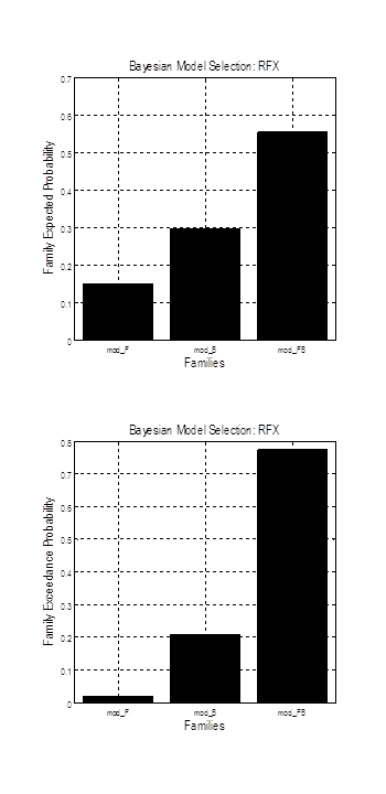
• Press the green button to run BMS. After several seconds, you should see a new plot with expected probability and exceedance probability for each family of models. Exceedance probability is the probability of each model being better than any other model. In the plot below on the left, you can see that the models with both forward and backward connections modulated by face presentation have higher evidence than the remaining models. The plot on the right shows single models.

Parameter inference

• First, you can inspect a single model from a single participant using the GUI. To do this, in Matlab go to the “pre-computed” directory, and in the GUI load one of Subject 15’s inverted models. Then use the drop-down menu in the lower left corner of the “DCM for M/EEG” window to view the results. For example, selecting “ERPs (mode)” will plot the observed (dashed lines) and model-predicted (solid lines) responses for all experimental conditions and spatiotemporal modes you have modeled. “ERPs (sources)” will plot the activity modeled for each neuronal source, including its different neuronal populations – in case of an ERP neuronal model, the solid lines will represent superficial pyramidal cells which contribute most strongly to the measured signals. Further options include e.g., “Coupling (B)” which will show you posterior estimates of modulatory connectivity parameters (the B matrix), and “trial-specific effects” (see below) which will show you connection strengths for different conditions (here 100% represents the connection strength for the baseline condition). Finally, “Response (image)” will show you the model fits across all modeled time points and sensors. This is the end of our demo.

• To formally test whether your posterior parameter estimates are significant, you can use Bayesian parameter averaging (spm_dcm_average) of the winning model across all participants and inspect the posterior estimates and probabilities of parameters (e.g., DCM.Ep.B{1}(1,3) and DCM.Pp.B{1}(1,3) will give you the posterior estimate and probability of the strength of a forward modulatory connection from region 3 to region 1). In a random effects context, you can load the posterior estimates of parameters from single subjects’ DCM structures – here, this would be one value of DCM.Ep.B{1}(1,3) per subject – to perform a one-sample t-test.

More examples and tutorials can be found in the SPM12 manual.