workshop / practicalmeeg2022 / handson_artifacts /
Dealing with artifacts
This tutorial was written specifically for the PracticalMEEG workshop in Aix-en-Provence in December 2022 and is part of a coherent sequence of tutorials.
Introduction
In this tutorial, we will learn how to deal with artifacts in the data. We do have a more general tutorial on dealing with artifacts, which is followed by a tutorial on visual artifact rejection and a tutorial on automatic artifact rejection. In the remainder of this tutorial we will give a short background, which is followed by a specific look at the artifacts that are present in the specific data. The focus will not be on cleaning up the data, but rather on learning how artifacts can be detected and dealt with.
In the remaining tutorials on this dataset for the PracticalMEEG workshop the data for all subjects is not cleaned but processed as-is. As you will see, the MEG data does not have such a strong representation of the blinks and the beamformer source reconstruction which we do to end up with group statistics on the source-level will quite well suppress the contribution of the eye activity.
However, had we planned other types of analysis, such as connectivity, then dealing with the EOG and especially ECG artifacts would have been more important. Furthermore, to increase the sensitivity of finding the effects of interest, a cleanup of the data would have been good. However, for didactical reasons, and since we don’t have the time for a complete and thorough analysis of all 16 subjects, we will not deal with artifacts outside of this tutorial. This tutorial demonstrates on the basis of subject 1 how we can detect and deal with artifacts; following this tutorial you may want to go back to computing ERPs/ERFs and look how the cleaning affects the results.
Since the data is very large, with more than 400 channels at 1100Hz for a total recording duration of 50 minutes, the strategy that we follow is to first define the segments with ft_definetrial and then only reading the segments of interest with ft_preprocessing.
An alternative strategy that often is preferred for smaller datasets that completely fit in memory of your computer is to read in the continuous data using ft_preprocessing and only later to cut out the segments of interest using ft_definetrial ft_redefinetrial. That approach is explained in a separate tutorial.
There are some differences between first segmenting and then detecting artifacts or detecting the artifacts in the continuous representation of the data. An important difference is that when you only look at segments of interest (aka trials), you won’t see artifacts that happen in between the trials. It might be that you instructed your participant to blink whenever there is no fixation cross on the screen, or that you allowed your participant some time to relax (and possibly some movement) in between blocks in your experiment. When only looking at the segments of interest, you won’t see (and probably won’t care) the corresponding artifacts.
When you process the data continuously, you may see artifacts at the start of the recording but prior to the start of the actual experiment when the subject is still moving around. You may also see other movement related artifacts at time windows when the subject was not engaged in the task, for example between blocks. With a continuous representation of the data you will also see more eye blinks and movements, which can be beneficial to improve the quality of the ICA decomposition.
Background
There are different causes for artifacts in the data, for example the subject might have blinked or moved, EEG channels might change their signal quality over time due to drying up of the gel, or MEG channels can have SQUID jumps.
Sometimes artifacts are restricted to a single channel, or to a short time window. In other cases artifacts can extend over all channels, or are present during the complete recording.
Artifacts due to external influences or instrumentation
These for example include 50Hz or 60Hz line noise, electrodes with poor impedance, sudden jumps in the MEG signal due to SQUID instabilities (so called SQUID jumps). In general these are always unwanted and also uninteresting. However, understanding the cause of the artifact can help us to make good decisions on how to deal with it during data analysis, or how to prevent them from happening in future experiments.
There can be situations where the external artifacts are influenced by behaviour, for example the amount of line noise that is picked up by the body (which acts as antenna) can be influenced by the position of the body and hence might change dependent on the participant’s movements. Also the presence of magnetic artifacts and SQUID jumps in the MEG can get worse if the participant has for example a magnetized magnetic wire behind the teeth.
Artifacts due to behaviour or physiology
These are for example due to the contribution of sources that we as neuroscientists in general are not interested in, such as the regular contraction of the heart muscle, the contraction of muscles in the neck and clenching of the jaws, movements of the tongue, movements of the eyes. Each of these causes electrophysiological contributions to the EEG or MEG signal; you should however consider that your noise may be someone else’s signal, e.g., a cardiologist will consider the ECG as the most interesting feature of the signal.
Sometimes it is difficult to say whether something is signal or noise, for example with interictal spikes in intracranial EEG (ECoG and sEEG) recordings: detecting and localizing the epilepsy is the reason why the iEEG electrodes were implanted in the first place, and the doctors mainly care about that part of the signal and hope that it will be well captured in the recordings. However, if the patient volunteered to participate in your experiment, you are likely not interested in the spikes and mostly care about the signal contributions from unaffected brain regions and cognitive processes.
Reading the raw data
We start with the raw data that we preprocessed in the previous tutorial
subj = datainfo_subject(1);
filename = fullfile(subj.outputpath, 'raw2erp', subj.name, sprintf('%s_data.mat', subj.name));
load(filename, 'data')
This data structure is about 1.5 GB large and should fit in the RAM of your computer.
>> whos data

  Name      Size                 Bytes  Class     Attributes
  data      1x1             1465245106  struct
The complete data represented in double precision would amount to approximately 50*60*1100*403*8 (50 minutes, times 60 seconds, times 1100 samples per second, times 403 channels, times 8 bytes per sample) is 10 GB and would most likely cause memory problems if you would process it using a laptop with limited memory.
Please have a look at the tutorial on making a memory efficient analysis pipeline for more information.
Looking for eye artifacts
The subject was performing a visual task, had to maintain fixation, and was (probably) instructed not to blink. The subject looking away or blinking during the presentation of a stimulus would not only contribute an EOG artifact to the EEG and MEG channels, but it might also affect the cortical processing of the stimulus itself.
Visual identification of eye artifacts
Since the data includes EOG channels, we can use those to identify the blinks and saccades. The ft_rejectvisual function has three methods: summary, trial and channel. When we use the method channel, we can visualize all trials for one channel:
cfg = [];
cfg.method = 'channel';
data_clean = ft_rejectvisual(cfg, data);
This function allows you to click on a trial to remove it from the data. It returns an updated data structure in which the excluded trials are removed.
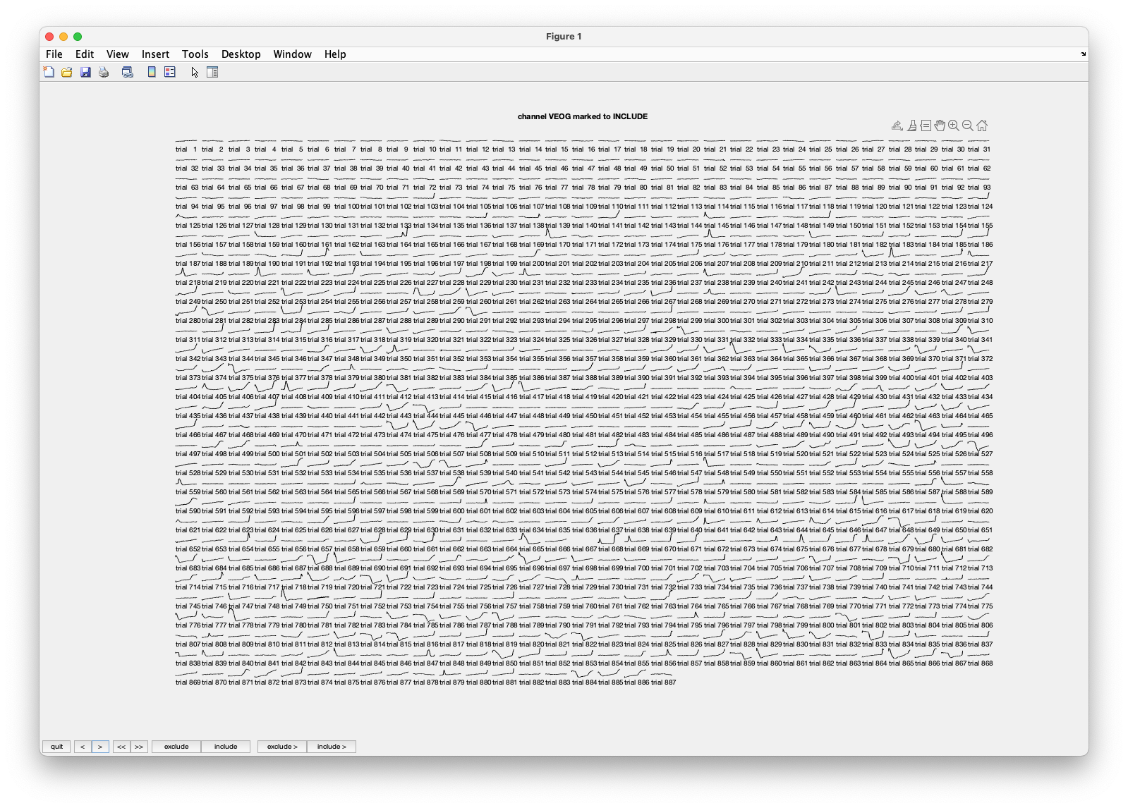
Figure; The single-trial responses for the VEOG channel
Besides there being many channels, there are also many trials. Visualizing them on a small computer screen might be hard. Remember: if you are working with large data, you better use a large computer (screen, memory, disk).
Please scroll to the VEOG channel by clicking about 40 times on the >> button which takes you 10 channels further and then clicking a few times on the > or < button. The EOG channels are located after all EEG channels, and before the STI channels. You can see that there are quite some blinks. You can also recognize that in the first 100 trials or so there are very few blinks, but that after trial 200 or so they start occuring more frequently. Remember that there are about 100 trials per block/run, and there are 6 runs in total.
If you click two channels further to the ECG channel, you can also see that there is a heartbeat (and sometimes two) in every trial. That is a good sign: the participant is alive! This makes directly clear that rejecting trials that contain a heartbeat does not make sense. We will later look at removing the heartbeat artifacts using ICA.
We might want to decide that we want to exclude trials with blinks from further analysis. You can click on trials to exclude. However, you will realize that this involves a lot of clicking, as there are so many trials. In the next section we will automate the detection of blinks, but for now please select a few trials with blinks and click quit. This returns a data structure with slightly fewer trials. However, it also specifies where the artifacts were that you identified:
>> disp(data_clean.cfg.artfctdef.channel.artifact)
       71401       71910
       73441       73950
       83131       83640
       86191       86700
       89251       89760
      112201      112710
This artifact matrix is very comparable to the trl matrix that ft_definetrial returns. In this case it contains the begin and endsample of each artifact that was detected using the “channel” method in ft_rejectvisual.
Had the data structure contained the sampleinfo field with a specification how each trial maps onto the continuous recording on disk, then the artifacts would have been expressed relative to the recording on disk. This allows for the same visual/manual identification of artifacts to be used repeatedly, even if you do the preprocessing again and for example extend the pre- or post-stimulus time a bit.
In this case you may have noticed “Warning: reconstructing sampleinfo by assuming that the trials are consecutive segments of a continuous recording”. This indicates that the original sampleinfo is not present, hence the artifacts are expressed relative to the data in memory.
In this case the original sampleinfo is not present since the data was compiled over 6 files on disk. Furthermore, the data was resampled from 1100 to 300 Hz, so the samples that we now work with do not map back to the files on disk.
Finding the EOG channels in between the 400 other channels is annoying. We can use the following code to make a data structure that only contains the EOG channels and use that to identify artifacts.
cfg = [];
cfg.channel = 'EOG';
data_eog = ft_selectdata(cfg, data);

cfg = [];
cfg.method = 'channel';
data_eog_clean = ft_rejectvisual(cfg, data_eog);
Again the output data excludes those trials that were rejected, however we don’t want to reject them only for the OEG channels, we want to reject them for the complete MEG+EEG data structure. For that we can use the list of artifact that was detected
>> disp(data_eog_clean.cfg.artfctdef.channel.artifact)
       26011       26520
       73441       73950
       83131       83640
       86191       86700
       89251       89760
      108631      109140
      154021      154530
      339661      340170
      ...

% remove the marked segments from the complete MEG+EEG data structure
cfg = [];
cfg.artfctdef = data_eog_clean.cfg.artfctdef; % use the artifacts that we just identified
data_all_clean = ft_rejectartifact(cfg, data);
Automatic identification of eye artifacts
FieldTrip also includes functions for the automatic identification of certain artifact types. The ft_artifact_eog function can be used to detect eye blinks and movements.
cfg = [];
cfg.artfctdef.eog.channel = 'EOG';
cfg.artfctdef.eog.interactive = 'yes';
cfg = ft_artifact_eog(cfg, data);
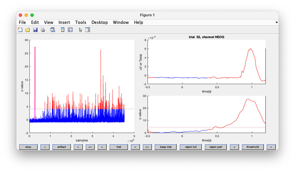
Figure; Automatic detection of artifacts using the EOG channels
Rather than returning a cleaned-up data structure, this function returns a configuration structure that details where the artifacts are located
>> disp(cfg.artfctdef.eog.artifact)
      26011       26041
      26267       26520
      73441       73528
      83465       83640
      86191       86362
      89322       89457
      ...
You can see that it identified many blinks. As before, we can use the detected blinks to remove the affected segments from the data.
% remember it for later inspection
cfg_automatic_eog.artfctdef = cfg.artfctdef;

% remove the marked segments
cfg.artfctdef.reject = 'complete';
data_clean = ft_rejectartifact(cfg, data);
The EOG detection above makes use of ft_artifact_zvalue, which filters, transforms and combines channels. This is especially useful in cases the artifacts are visible on many channels. We can also use it on the EEG channels, or on the frontal MEG channels. The procedure is explained in more detail here
Exercise 1
Using the following code, use all EEG channels instead of the dedicated EOG channels to identify the eye artifacts.
cfg = [];
cfg.artfctdef.eog.channel = 'EEG';  % use the EEG channels to detect eye artifacts
cfg.artfctdef.eog.interactive = 'yes';
cfg.artfctdef.eog.cutoff = 20;
cfg = ft_artifact_eog(cfg, data);
The artifact score is computed by preprocessing each channel, z-transforming it,and summing over all channels. Therefore it depends on the number of channels that “see” the artifact. Consequently, a different threshold is needed for the cutoff depending on the number of channels. Are you finding the same artifacts as before?
Simple thresholding to identify artifacts
Since we have the two EOG channels, we don’t need a fancy combination of z-values, but we can also simply threshold the EOG channels using ft_artifact_threshold.
cfg = [];
cfg.artfctdef.threshold.channel = 'EOG';
cfg.artfctdef.threshold.demean = 'yes';
cfg.artfctdef.threshold.min = -100 * 1e-6;
cfg.artfctdef.threshold.max =  100 * 1e-6;
cfg.artfctdef.threshold.bpfilter = 'no';
cfg = ft_artifact_threshold(cfg, data);
The way that the output represents the segments that were marked is the same as before, except that it now also includes an offset of the peaks. This can be useful if you want to align and process the artifacts specifically, for example if you want to compute an averaged eye blink or ECG template.
>> disp(cfg.artfctdef.threshold.artifact)
       26419       26419           0
       26426       26484         -28
       26500       26520          -9
       52517       52530         -13
       63221       63240         -19
       63290       63316         -12
       69337       69360         -12
       70348       70365          -6
       ...

% remember it for later inspection
cfg_automatic_threshold.artfctdef = cfg.artfctdef;

% remove the marked segments
cfg.artfctdef.reject = 'complete';
data_clean = ft_rejectartifact(cfg, data);
Inspect and update the marked artifacts
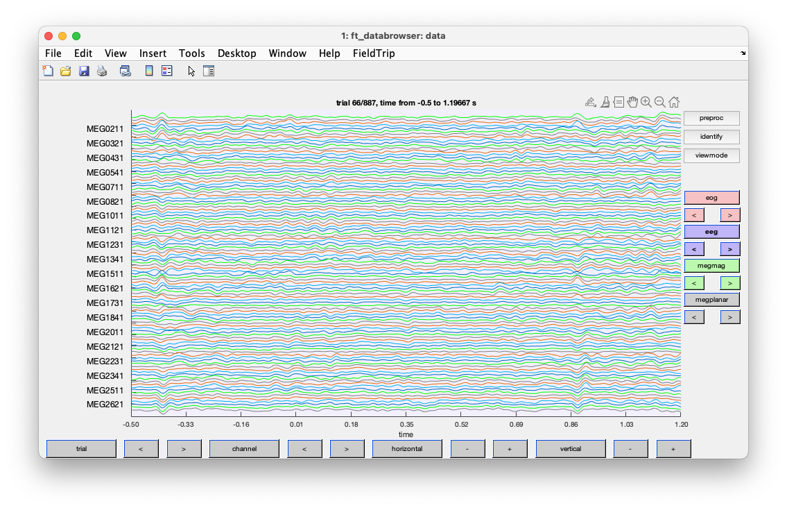
We can use the ft_databrowser function to inspect the data. It can also be used to mark visually identified artifacts.
cfg = [];
cfg.channel = 'EOG';
cfg = ft_databrowser(cfg, data);
You should reduce the vertical shale, and go to trial 125. If you click with your left mouse button, you can drag and make a selection. If you subsequently click in that selection, you can mark the segment as an artifact.
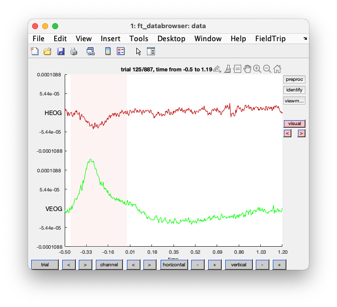
Figure; ft_databrowser shows an artifact in the EOG channels
The output cfg structure again contains the segments that you marked as artifacts, and using ft_rejectartifact you could remove those segments from the data.
Since there are many trials (about 800 in total), going through all of them can be rather time consuming. We can also pretend that the data is continuous and show more data at the time.
cfg = [];
cfg.channel = 'EOG';
cfg.continuous = 'yes';
cfg.blocksize = 30;
cfg.ylim = [-200 200]*1e-6;

% to get you started here are some that I marked
cfg.artfctdef.visual.artifact = [
       52484       52546
       63142       63542
       67315       67479
       69299       69409
       70303       70388
       70877       70993
       71821       71961
       73430       73540
       75916       76014
       80548       80682
       ];

cfg = ft_databrowser(cfg, data);
Along the horizontal axes you now see 30 seconds of data. Note that the data is in reality not continuous and that you might see some small jumps at the boundaries between trials. You can now horizontally zoom in or out to a convenient time scale. If you jump to about 300 seconds in the data, you can see that the blink frequency is increasing. Again, marking all of those blinks would be a lot of work.
We can also use the automatically identified artifact segments and visualize them in ft_databrowser.
cfg = [];
cfg.channel = 'EOG';
cfg.continuous = 'yes';
cfg.blocksize = 30;
cfg.ylim = [-200 200]*1e-6;

% reuse the automatic artifacts from above
cfg.artfctdef.eog       = cfg_automatic_eog.artfctdef.eog;
cfg.artfctdef.threshold = cfg_automatic_threshold.artfctdef.threshold;

% inspect and adjust the marked segments
cfg = ft_databrowser(cfg, data);
After we are done with adding, removing and/or updating the marked artifacts, we can remove them from the data.
% remove the marked segments
data_clean = ft_rejectartifact(cfg, data);
Using the summary mode to remove artifacts
The ft_rejectvisual function that we used before with the channel mode also has the trial and the summary mode. The summary mode can be very efficient in quickly processing large amounts of data. It computes a summary metric (for example the variance) for every channel and every trial and displays that. Furthermore, it displays the maximum variance over all channels, and the maxium variance over all trials. That allows you to quickly identify trials or channels with large variance, which is indicative of there being an artifact. The function is explained in more detail here.
In this case we have very different channel types with very different units (V, T, T/m), which makes the variance not comparable over the channels. We could use the cfg.eegscale, cfg.gradscale and cfg.magscale options to make the channels more numerically comparable, however here we will just look at the different channel types sequentially.
cfg = [];
cfg.method = 'summary';
cfg.channel = 'EOG';
cfg.keepchannel = 'yes';
data_clean = ft_rejectvisual(cfg, data);
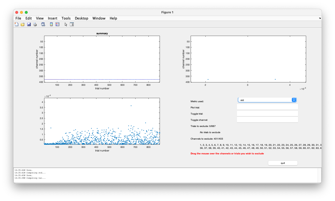
Figure; ft_rejectvisual with the summary method applied to the EOG channels
This shows the variance of the EOG channels. You can switch to the std or standard-deviation metric, which is slightly easier to understand. In the lower left you see the maximum over the HEOG and VEOG channel. It ranges up to 4e-4 or 4*10^-4 volt, which corresponds to 400 microvolt.
A realistic range for the background activity and noise in the EOG channels if there are no blinks or saccades is a standard deviation in the order of magnitude of 20 microvolt: that is what we see in the trials of the first block. We can drag and select trials to exclude. If we reject all trials with a standard deviation in the EOG channels larger than 20 microvolt, we see that “361 trials are marked to INCLUDE, 526 trials are marked to EXCLUDE”, i.e., we loose more than half of the trials.
Exercise 2
Use the same approach on the EEG channels. The EEG channels have a different spacing to the reference electrode and different signal amplitudes. What threshold is realistic for the standard deviation of the EEG channels?
It is a bit annoying that there are so many channels (EEG, magnetometers, planar gradiometers, EOG, misc) and that the color-coded display of the metric has very little detail if we only look at a small set of the channels. We can use the same strategy we used before to select the channels, to look at them and identify artifacts, and to combine all the artifacts afterwards.
cfg = [];
cfg.channel = 'eog';
data_eog = ft_selectdata(cfg, data);

cfg = [];
cfg.method = 'summary';
cfg.keepchannel = 'yes';
data_eog_clean = ft_rejectvisual(cfg, data_eog);

cfg = [];
cfg.channel = 'EEG*';  % 'eeg' as such is not recognized
data_eeg = ft_selectdata(cfg, data);

cfg = [];
cfg.method = 'summary';
cfg.keepchannel = 'yes';
data_eeg_clean = ft_rejectvisual(cfg, data_eeg);

cfg = [];
cfg.channel = 'megmag';
data_megmag = ft_selectdata(cfg, data);

cfg = [];
cfg.method = 'summary';
cfg.keepchannel = 'yes';
data_megmag_clean = ft_rejectvisual(cfg, data_megmag);

cfg = [];
cfg.method = 'summary';
cfg.channel = 'megplanar';
data_megplanar = ft_selectdata(cfg, data);

cfg = [];
cfg.method = 'summary';
cfg.keepchannel = 'yes';
data_megplanar_clean = ft_rejectvisual(cfg, data_megplanar);
For each of the channel types, the magnitude of the metric is different and especially the magnitude for the magnetometer channels (in T) and planar gradiometer channels (in T/m) is very different. However, the pattern of artifacts is very clear. We can combine all artifacts that we identified so far and remove them from the original data.
cfg = [];

% rename the artifacts to the corresponding channel types
cfg.artfctdef.eog.artifact       = data_eog_clean.cfg.artfctdef.summary.artifact;
cfg.artfctdef.eeg.artifact       = data_eeg_clean.cfg.artfctdef.summary.artifact;
cfg.artfctdef.megmag.artifact    = data_megmag_clean.cfg.artfctdef.summary.artifact;
cfg.artfctdef.megplanar.artifact = data_megplanar_clean.cfg.artfctdef.summary.artifact;

% inspect and adjust the marked segments
cfg.channel = 'megmag'; % look only at the 102 magnetometers
cfg = ft_databrowser(cfg, data);

% remove the marked segments
cfg = rmfield(cfg, 'channel'); % this is not an option for ft_rejectartifact
data_clean = ft_rejectartifact(cfg, data);
Figure; ft_databrowser shows the magnetometer channels and all identified artifacts
A closer look at when the artifacts happen
The eye artifacts are not merely a nuisance to the EEG and MEG signal of interest, they also convey information about the behavior of the participant. It is therefore relevant to know what the behaviour is.
We have already observed that the amount of eye blinks increases considerably after the first trial. This is something that we might want to quantify and consider whether this has confounding effects on our analysis and interpretation of the results. For example if there is a learning component in the experiment, and if the number of eye blinks increases over time, there could be a systematic increase in low-frequency contributions to the signal. The removal of eye artifacts is likely not to be perfect and hence you would expect it to remain as a confound. Furthermore, even when you remove the overt eye artifacts in such a case, you would still not be sure whether there would not be an increase in (covert) brain activity that causes the participant to make those movement does not remain a confound.
The same consideration holds when identifying heartbeats; an increase in the number of heartbeats (which is best identified in the continuous data) and thereby the heart rate can indicate that the subject is getting more anxious or stressed, again something to consider as a potential confounding effect in your experimental design.
In which trials are the artifacts?
Using the following code we can count how many trials we originally had in each condition, and how many are remaining.
% this is what we can see in the BIDS events.tsv file
Famous      = [5 6 7];
Unfamiliar  = [13 14 15];
Scrambled   = [17 18 19];

sum(ismember(data.trialinfo, Famous))
sum(ismember(data.trialinfo, Unfamiliar))
sum(ismember(data.trialinfo, Scrambled))

sum(ismember(data_clean.trialinfo, Famous))
sum(ismember(data_clean.trialinfo, Unfamiliar))
sum(ismember(data_clean.trialinfo, Scrambled))
Exercise 3
Is there a reason to believe that this participant was blinking more in the faces than in the scrambled faces condition? Do you think there is a confounding effect of the behaviour of the participant on the contrast of interest?
Where in the experiment are the artifacts?
We already noticed that there are fewer blinks at the start and more toward the end. That is something we can quantify in more detail.
We can construct a single vector that represents all samples in the experiment and give that the value 0 if there is no artifact, or 1 if there is. We first need to count the total number of samples:
nsamples = sum(cellfun(@length, data.trial));

% make a vector with a zero for every sample
artifact = zeros(1, nsamples);

% compute the time in the experiment, this does not account for the time between trials or runs
time = ((1:nsamples)-1)/data.fsample;
Now we can use the identified artifacts and replace the 0 by a 1.
for i=1:size(cfg_automatic_threshold.artfctdef.threshold.artifact, 1)
  begsample = cfg_automatic_threshold.artfctdef.threshold.artifact(i,1);
  endsample = cfg_automatic_threshold.artfctdef.threshold.artifact(i,1);
  artifact(begsample:endsample) = 1;
end

% plot where in time in the experiment the artifacts happen
plot(time, artifact)

% make a smooth representation of where in time the artifacts happen
% this smoothes with 3000 samples, which is 10 seconds
plot(time, conv(artifact, ones(1,3000), 'same'))
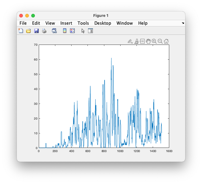
Figure; Increasing occurence of artifacts over time in the experiment
It would be possible to cut this smoothed vector of artifact occurence up into trials and to add it to the data structure. That would allow statistically testing later on in the analysis whether the difference in experimental conditions is reflected in a difference in the number of artifacts, a strong indicator of the artifacts causing a confounding effect.
A similar strategy can be used to detect the heartbeats and to determine the heartrate. The ft_heartrate function can be used for this, by preference on the continuous representation of the ECG channel. The extracted heart rate (which is represented as a continuous channel) can be segmented using ft_redefinetrial and combined with the EEG and MEG using ft_appenddata. This allows the same type of statistical analysis to be performed on the heartrate and to determine whether an increase in heartrate might be responsible for a spurrious increase in connectivity that would be estimated between brain regions.
Besides ft_heartrate, you may want to look at ft_headmovement and ft_regressconfound and this example script. For the purpose of the hands-on during the workshop it is fine to skip this for now.
Where are the artifacts relative to the stimulus?
Using the previously determined cfg_automatic_threshold, which does not mark trials but only those parts of the trial where the signal exceeds the threshold, we can also check where the artifact happens within the trial. For that we are not going to reject the artifacts, but we will replace it with a NaN (not a number) value and count over trials how many of those we have for each time point.
cfg = [];
cfg.channel = 'VEOG'; % a single channel is enough
data_eog = ft_selectdata(cfg, data);

cfg = [];
cfg.artfctdef = cfg_automatic_threshold.artfctdef;
cfg.artfctdef.reject = 'nan';
data_artifact = ft_rejectartifact(cfg, data_eog);

for i=1:numel(data_artifact.trial)
  % find where the nans are in every trial
  data_artifact.trial{i} = isnan(data_artifact.trial{i});
end

cfg = [];
avg_artifact = ft_timelockanalysis(cfg, data_artifact);

plot(avg_artifact.time, avg_artifact.avg);
xlabel('time (s)')
ylabel('fraction between 0 and 1')
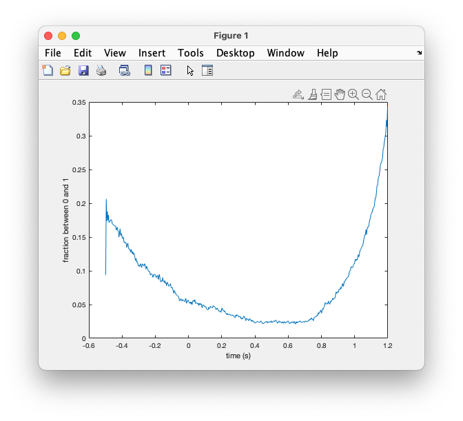
Figure; Occurence of artifacts over time in the trial, i.e., relative to the stimulus
It is clear that most blinks happened at the start and especially towards the end of the trial. Looking at this, we can conclude that the participant was trying to suppress their blinks during stimulus presentation. It is not likely that the frequent eye blinks will have affected the perception of the stimulus as a (famous or unfamiliar) face, or as a scrambled object.
Removing the eye and heart artifacts
Rather than excluding the data segments affected by artifacts from further analysis, we can also subtract the contribution of the artifacts from the data. This is in principle the same as what we do when we apply a band-stop filter to remove the line noise.
The strategy for this is to use ft_componentanalysis to make an ICA composition. By inspecting the component topographies and time courses we can identify which components reflect the artifacts. Using ft_rejectcomponent we can back-project the components back to the channels, minus those components that capture the artifactual signal contributions.
Note that ICA assumes a stationary mixing of all the (brain and artifact) sources to the channels. If the subject moves their head it will not affect the EEG, as the electrodes are attached to the scalp, but may affect the MEG topographies. The spatial sensitivity of the EEG, and the planar and gradiometer MEG channels will also be different. Nevertheless, we do expect all three channel types to pick up some signatures of the EOG and ECG artifacts.
Exercise 4
Use ft_componentanalysis and ft_rejectcomponent to remove the eye- and heart-related artifacts from the EEG and the MEG data.
You can follow the tutorial on cleaning artifacts in MEG data using ICA.