SPED4 - Time-frequency analysis in practice using FieldTrip

Introduction

This is an adapted version of the general FieldTrip tutorial on time-frequency analysis, made specifically for the module Signal Processing for Electrophysiological Data (SPED) in the course Neuroimaging 2: Electrophysiological Methods, in the Cognitive Neuroscience Masters (CNS) program at Radboud University. This module is taught by Eelke Spaak.

Some of the concepts convered here should by now be familiar to you, while some other concepts will be new. The main purpose of this week’s tutorial is to show you how spectral and time-frequency data analysis is done when using a typical, widely used, analysis toolbox. This is in contrast to previous weeks, in which the focus was much more on implementing the basic methods yourself and understanding their intricacies. Specifically, this tutorial will cover the time-frequency analysis of a single subject’s MEG data using a Hanning window, multitapers and wavelets. The tutorial also shows how to visualize the results.

Please collect all the code you write for this tutorial in a single MATLAB live script file, which you can hand in via Brightspace. Ensure that your answers to the exercises are in separate text or code cells with clear labels (“Exercise 1” etc. in bold face will do). Also please start new code cells in your live script for each snippet of code provided here in the tutorial. You can break up a code cell by typing three dashes on a code line (---). Make sure all code cells are executed and the relevant plots are embedded.

Details on the dataset

The MEG data set used here is from a language study on semantically congruent and incongruent sentences that is described in detail in Wang et al. (2012). Three types of sentences were used in the experiment. In the fully congruent condition (FC) the sentences ended with a high-cloze probability word, e.g., De klimmers bereikten eindelijk de top van de berg (The climbers finally reached the top of the mountain) In the fully incongruent condition (FIC) sentences ended with a semantically anomalous word which was totally unexpected given the sentential context, e.g., De klimmers bereikten eindelijk de top van de tulp (The climbers finally reached the top of the tulip). The third type of sentences ended with a semantically anomalous word that had the same initial phonemes (and lexical stress) as the high-cloze words from the congruent condition: initially congruent (IC). There were 87 trials per condition for each of the three conditions, and a set of 87 filler sentences were added. From the EEG literature it is known that a stronger negative potential is produced following incongruent compared to congruent sentence endings about 300-500 ms after the word onset. This response is termed the N400 effect¹ ². For more information about the materials you could take a look at the published EEG experiment using the same sentence materials³.

In the study applied here, the subjects were seated in a relaxed position under the MEG helmet. Their task was to attentively listen to spoken sentences. They were informed that some of the sentences would be semantically anomalous. Acoustic transducers were used to deliver the auditory stimuli. After a 300-ms warning tone, followed by a 1200 ms pause, a sentence was presented. Every next trial began 4100 ms after the offset of the previous sentence. To reduce eye blinks and movements in the time interval in which the sentence was presented, subjects were instructed to fixate on an asterisk presented visually 1000 ms prior to the beginning of the sentence. The asterisk remained on the screen until 1600 ms after the onset of the spoken sentence. Subjects were encouraged to blink when the asterisk was not displayed on the screen.

MEG signals were recorded with a 151-channel CTF system. In addition, the EOG was recorded to later discard trials contaminated by eye movements and blinks. The ongoing MEG and EOG signals were lowpass filtered at 100 Hz, digitized at 300 Hz and stored for off-line analysis. To measure the head position with respect to the sensors, three coils were placed at anatomical landmarks of the head (nasion, left and right ear canal). While the subjects were seated under the MEG helmet, the positions of the coils were determined before and after the experiment by measuring the magnetic signals produced by currents passed through the coils.

The MEG data are stored as epochs or trials of fixed length around each stimulus trigger.

There is no information in this tutorial about how to compare conditions, how to grandaverage the results across subjects or how to do statistical analysis on the time-frequency data. Some of these issues are covered in other tutorials (see the summary and suggested further reading section).

Background on time-frequency analysis

Oscillatory components contained in the ongoing EEG or MEG signal often show power changes relative to experimental events. These signals are not necessarily phase-locked to the event and will not be represented in event-related fields and potentials (Tallon-Baudry and Bertrand (1999)). The goal of this section is to compute and visualize event-related changes by calculating time-frequency representations (TFRs) of power. This will be done using analysis based on Fourier analysis and wavelets. The Fourier analysis will include the application of multitapers (Mitra and Pesaran (1999), Percival and Walden (1993)) which allow a better control of time and frequency smoothing.

Calculating time-frequency representations of power is done using a sliding time window. This can be done according to two principles: either the time window has a fixed length independent of frequency, or the time window decreases in length with increased frequency. For each time window the power is calculated. Prior to calculating the power one or more tapers are multiplied with the data. The aim of the tapers is to reduce spectral leakage and control the frequency smoothing.

Figure: Time and frequency smoothing. (a) For a fixed length time window the time and frequency smoothing remains fixed. (b) For time windows that decrease with frequency, the temporal smoothing decreases and the frequency smoothing increases.

If you want to know more about tapers/ window functions you can have a look at this Wikipedia site. Note that Hann window is another name for Hanning window used in this tutorial. There is also a Wikipedia site about multitapers, to take a look at it click here.

Procedure

To calculate the time-frequency analysis for the example dataset we will perform the following steps:

• Read the data into MATLAB using ft_definetrial and ft_preprocessing
• Seperate the trials from each condition using ft_selectdata
• Compute the power values for each frequency bin and each time bin using the function ft_freqanalysis
• Visualize the results. This can be done by creating time-frequency plots for one (ft_singleplotTFR) or several channels (ft_multiplotTFR), or by creating a topographic plot for a specified time- and frequency interval (ft_topoplotTFR).

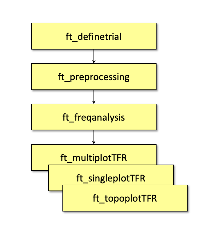
Figure: Schematic overview of the steps in time-frequency analysis

In this tutorial, procedures of 4 types of time-frequency analysis will be shown. You can see each of them under the titles: Time-frequency analysis I, II … and so on. If you are interested in a detailed description about how to visualize the results, look at the visualization part.

Preprocessing

The first step is to read the data using the function ft_preprocessing. It is recommended to read larger time intervals than the time period of interest. In this example, the time of interest is from -0.5 s to 1.5 s (t = 0 s defines the time of stimulus); however, the script reads the data from -1.0 s to 2.0 s.

Reading in the data

First, download the data from here and unzip it somewhere. Make sure FieldTrip is added to your MATLAB path:

addpath <wherever FieldTrip lives>
ft_defaults

Then, execute the following code, which will determine the time indices of the trials of interest (note: adapt the path to wherever you unzipped Subject01.ds):

cfg                         = [];
cfg.dataset                 = '<path>/Subject01.ds';
cfg.trialfun                = 'ft_trialfun_general'; % this is the default
cfg.trialdef.eventtype      = 'backpanel trigger'; % name of the trigger channel in the dataset
cfg.trialdef.eventvalue     = [3 5 9]; % the values of the stimulus trigger for the three conditions
% 3 = fully incongruent (FIC), 5 = initially congruent (IC), 9 = fully congruent (FC)
cfg.trialdef.prestim        = 1; % in seconds
cfg.trialdef.poststim       = 2; % in seconds

cfg = ft_definetrial(cfg);

The resulting cfg structure will have a cfg.trl matrix which contains the begin and end samples of all trials of interest, as well as the offset (3rd column) that determines which sample corresponds to time points t = 0.

Cleaning

Some trials have previously been identified as artifactual (due to for example eye blinks or MEG SQUID jumps). Also, two MEG channels were malfunctioning. Both these trials and channels need to be removed. Furthermore, while reading in the data, we remove the overall per-trial and per-channel mean to facilitate downstream time-frequency analysis. The following code achieves all this and reads in the data:

% remove the trials that have artifacts from the trl
cfg.trl([2, 5, 6, 8, 9, 10, 12, 39, 43, 46, 49, 52, 58, 84, 102, 107, 114, 115, 116, 119, 121, 123, 126, 127, 128, 133, 137, 143, 144, 147, 149, 158, 181, 229, 230, 233, 241, 243, 245, 250, 254, 260],:) = [];

% preprocess the data
cfg.channel   = {'MEG', '-MLP31', '-MLO12'};        % read all MEG channels except MLP31 and MLO12
cfg.demean    = 'yes';                              % do baseline correction with the complete trial

data_all = ft_preprocessing(cfg);

We now select one of the conditions from the dataset for time-frequency analysis:

cfg = [];
cfg.trials = data_all.trialinfo == 3;
dataFIC = ft_redefinetrial(cfg, data_all);

If you want, you can save the data to disk in order to easily continue later on, without having to read in all data again:

save dataFIC dataFIC

TFR I: Hanning taper, fixed window length

Here, we will describe how to calculate time frequency representations using the commonly used Hanning, or Hann, tapers. When choosing for a fixed window length procedure, the frequency resolution is defined according to the length of the time window (delta T). The frequency resolution (delta f in figure 1) = 1/length of time window in sec (delta T in figure 1). Thus a 500 ms time window results in a 2 Hz frequency resolution (1/0.5 sec = 2 Hz) meaning that power can be calculated for 2 Hz, 4 Hz, 6 Hz etc. An integer number of cycles should fit in the time window.

In the following example, a time window with length 500 ms is applied:

cfg              = [];
cfg.output       = 'pow';
cfg.channel      = 'MEG';
cfg.method       = 'mtmconvol';
cfg.taper        = 'hanning';
cfg.foi          = 2:2:30;                         % analysis 2 to 30 Hz in steps of 2 Hz
cfg.t_ftimwin    = ones(length(cfg.foi),1).*0.5;   % length of time window = 0.5 sec
cfg.toi          = -0.5:0.05:1.5;                  % time window "slides" from -0.5 to 1.5 sec in steps of 0.05 sec (50 ms)
TFRhann = ft_freqanalysis(cfg, dataFIC);

The field cfg.method = 'mtmconvol'; instructs ft_freqanalysis to execute a convolution-type analysis. (The “mtm” stands for “multitaper method”, which will be explained in more detail below, but is mainly there for historical reasons, since the function also supports convolution that is not based on multitapers.) Regardless of the method used for calculating the TFR, the output format is identical. It is a structure with the following fields:

TFRhann =
        label: {149x1 cell}                % Channel names
       dimord: 'chan_freq_time'            % Dimensions contained in powspctrm, channels X frequencies X time
         freq: [2 4 6 8 10 12 14 16 18 20 22 24 26 28 30]  % Array of frequencies of interest (the elements of freq may be different from your cfg.foi input depending on your trial length)
         time: [1x41 double]               % Array of time points considered
    powspctrm: [149x15x41 double]          % 3-D matrix containing the power values
         elec: [1x1 struct]                % Electrode positions etc
         grad: [1x1 struct]                % Gradiometer positions etc
          cfg: [1x1 struct]                % Settings used in computing this frequency decomposition

The field TFRhann.powspctrm contains the temporal evolution of the raw power values for each specified frequency.

Visualization with standard MATLAB code

To facilitate understanding of the output of ft_freqanalysis, it is instructive to first plot it all in the same way we did before using imagesc. To do this, we need to first average over channels to obtain a 2D matrix.

pow_allchan = squeeze(mean(TFRhann.powspctrm, 1));
figure;
imagesc(TFRhann.time, TFRhann.freq, pow_allchan);
axis xy;
colorbar();
xlabel('time (s)');
ylabel('frequency (Hz)');

Visualization with FieldTrip code

As discussed in the videos and lecture, biological signals are often dominated by a strong so-called “1/f” component. In order to visualize and interpret task-related changes in oscillatory activity with respect to a baseline window, it is therefore recommended to perform baseline normalization.

In general there are two possibilities for normalizing:

• Subtracting, for each frequency, the average power in a baseline interval from all other power values. This gives, for each frequency, the absolute change in power with respect to the baseline interval.
• Expressing, for each frequency, the raw power values as the relative increase or decrease with respect to the power in the baseline interval. This means active period/baseline. If we furthermore log-transform (and scale) these ratios, we end up with the commonly used decibel (db).

There are three ways of graphically representing the data: 1) time-frequency plots of all channels, in a quasi-topographical layout, 2) time-frequency plot of an individual channel (or average of several channels), 3) topographical 2-D map of the power changes in a specified time-frequency interval.

To plot the TFRs from all the sensors use the function ft_multiplotTFR. Settings can be adjusted in the cfg structure. For example:

cfg = [];
cfg.baseline     = [-0.5 -0.1];
cfg.baselinetype = 'db'; % use db baseline correction
cfg.zlim         = 'maxabs'; % color scale symmetric around zero
cfg.showlabels   = 'yes';
cfg.layout       = 'CTF151_helmet.mat';
figure
ft_multiplotTFR(cfg, TFRhann);

Note that using the options cfg.baseline and cfg.baselinetype results in baseline correction of the data, implicitly during the plotting call. Baseline correction can also be applied explicitly by calling ft_freqbaseline. Moreover, you can combine the various visualization options/functions interactively to explore your data.

An interesting effect seems to be present in the TFR of sensor MRC15. To make a plot of a single channel use the function ft_singleplotTFR.

cfg = [];
cfg.baseline     = [-0.5 -0.1];
cfg.baselinetype = 'db';
cfg.zlim         = 'maxabs';
cfg.channel      = 'MRC15';
cfg.layout       = 'CTF151_helmet.mat';
figure
ft_singleplotTFR(cfg, TFRhann);

From the previous figure you can see that there is an increase in power around 15-20 Hz in the time interval 0.9 to 1.3 s after stimulus onset. To show the topography of the beta increase use the function ft_topoplotTFR.

cfg = [];
cfg.baseline     = [-0.5 -0.1];
cfg.baselinetype = 'db';
cfg.xlim         = [0.9 1.3];
cfg.zlim         = 'maxabs';
cfg.ylim         = [15 20];
cfg.marker       = 'on';
cfg.layout       = 'CTF151_helmet.mat';
cfg.colorbar     = 'yes';
figure
ft_topoplotTFR(cfg, TFRhann);

TFR II: Hanning taper, frequency dependent window length

It is also possible to calculate the TFRs with respect to a time window that varies with frequency. Typically the time window gets shorter with an increase in frequency. The main advantage of this approach is that the temporal smoothing decreases with higher frequencies, leading to increased sensitivity to short-lived effects. However, an increased temporal resolution is at the expense of frequency resolution.

We will here show how to perform a frequency-dependent time-window analysis, using a sliding window Hanning taper based approach. The approach is very similar to wavelet analysis. A wavelet analysis performed with a Morlet wavelet mainly differs by applying a Gaussian shaped taper (see Time-frequency analysis IV).

The analysis is best done by first selecting the numbers of cycles per time window which will be the same for all frequencies. For instance if the number of cycles per window is 7, the time window is 1000 ms for 7 Hz (1/7 x 7 cycles); 700 ms for 10 Hz (1/10 x 7 cycles) and 350 ms for 20 Hz (1/20 x 7 cycles). The frequency can be chosen arbitrarily - however; too fine a frequency resolution is just going to increase the redundancy rather than providing new information.

Below is the configuration for a 7-cycle time window. The calculation is only done for one sensor (MRC15) but it can of course be extended to all sensors.

cfg              = [];
cfg.output       = 'pow';
cfg.channel      = 'MRC15';
cfg.method       = 'mtmconvol';
cfg.taper        = 'hanning';
cfg.foi          = 2:1:30;
cfg.t_ftimwin    = 7./cfg.foi;  % 7 cycles per time window
cfg.toi          = -0.5:0.05:1.5;
TFRhann7 = ft_freqanalysis(cfg, dataFIC);

To plot the result use ft_singleplotTFR:

cfg              = [];
cfg.baseline     = [-0.5 -0.1];
cfg.baselinetype = 'db';
cfg.zlim         = 'maxabs';
cfg.channel      = 'MRC15';
cfg.interactive  = 'no';
cfg.layout       = 'CTF151_helmet.mat';
figure
ft_singleplotTFR(cfg, TFRhann7);

TFR III: Morlet wavelets

As discussed in detail in the videos, lectures, and last week’s assignment, a common way to calculate TFRs is convolution with Morlet wavelets. The approach is equivalent to calculating TFRs with sliding time windows that depend on frequency using a taper with a Gaussian shape.

The commands below illustrate how to do Morlet-wavelet based analysis in FieldTrip. One crucial parameter to set is cfg.width. It determines the width of the wavelets in number of cycles. Making the value smaller will increase the temporal resolution at the expense of frequency resolution and vice versa. The spectral bandwidth at a given frequency F is equal to F/width*2 (so, at 30 Hz and a width of 7, the spectral bandwidth is 30/7*2 = 8.6 Hz) while the wavelet duration is equal to width/F/pi (in this case, 7/30/pi = 0.074s = 74ms) (Tallon-Baudry and Bertrand (1999)).

Calculate TFRs using Morlet wavelet convolution:

cfg = [];
cfg.channel    = 'MEG';
cfg.method     = 'wavelet';
cfg.width      = 7;
cfg.output     = 'pow';
cfg.foi        = 1:2:30;
cfg.toi        = -0.5:0.05:1.5;
TFRwave = ft_freqanalysis(cfg, dataFIC);

Plot the result (again, recommended to do this in the command window directly because of interactive move):

cfg = [];
cfg.baseline     = [-0.5 -0.1];
cfg.baselinetype = 'db';
cfg.zlim         = 'maxabs';
cfg.showlabels   = 'yes';
cfg.layout       = 'CTF151_helmet.mat';
cfg.colorbar     = 'yes';
figure
ft_multiplotTFR(cfg, TFRwave)

TFR IV: Multitapers

Multitapers (literally: multiple tapers per time window of interest) are sometimes used in order to achieve better control over the frequency smoothing. More tapers for a given time window will result in stronger smoothing. For frequencies above 30 Hz, smoothing has been shown to be advantageous, increasing sensitivity thanks to reduced variance in the estimates despite reduced effective spectral resolution. Oscillatory gamma activity (30-100 Hz) is quite broad band and thus analysis of this signal component benefits from multitapering, which trades spectral resolution against increased sensitivity. For signals lower than 30 Hz it is recommend to use only a single taper, e.g., a Hanning taper as shown above (beware that in the example below multitapers are used to analyze low frequencies because there are no effects in the gamma band in this dataset).

Time-frequency analysis based on multitapers is also performed by ft_freqanalysis. The function uses a sliding time window for which the power is calculated for a given frequency. Prior to calculating the power by discrete Fourier transforms the data are ‘tapered’. Several orthogonal tapers might be used for each time window. The power is calculated for each tapered data segment and then combined. In the example below we apply a time window which gradually becomes shorter for higher frequencies (similar to wavelet techniques). Note that this is not necessary, but up to the researcher to decide. The arguments for the chosen parameters are as follows:

• cfg.foi, the frequencies of interest, here from 1 Hz to 30 Hz in steps of 2 Hz. The step size could be decreased at the expense of computation time and redundancy.
• cfg.toi, the time-interval of interest. This vector determines the center times for the time windows for which the power values should be calculated. The setting cfg.toi = -0.5:0.05:1.5 results in power values from -0.5 to 1.5 s in steps of 50 ms. A finer time resolution will give redundant information and longer computation times, but a smoother graphical output.
• cfg.t_ftimwin is the length of the sliding time-window in seconds. We have chosen cfg.t_ftimwin = 5./cfg.foi, i.e. 5 cycles per time-window. When choosing this parameter it is important that a full number of cycles fit within the time-window for a given frequency.
• cfg.tapsmofrq determines the width of frequency smoothing in Hz. We have chosen cfg.tapsmofrq = cfg.foi*0.4, i.e. the smoothing will increase with frequency. Specifying larger values will result in more frequency smoothing. For less smoothing you can specify smaller values, however, the following relation determined by the Shannon number must hold (see Percival and Walden (1993)): K = 2*tw*fw-1,

where K is required to be larger than 0. K is the number of tapers applied; the more, the greater the smoothing.

These settings result in the following characteristics as a function of the frequencies of interest:

Figure: a) The characteristics of the TFRs settings using multitapers in terms of time and frequency resolution of the settings applied in the example. b) Examples of the time-frequency tiles resulting from the settings.

cfg = [];
cfg.output     = 'pow';
cfg.channel    = 'MEG';
cfg.method     = 'mtmconvol';
cfg.foi        = 1:2:30;
cfg.t_ftimwin  = 5./cfg.foi;
cfg.tapsmofrq  = 0.4 *cfg.foi;
cfg.toi        = -0.5:0.05:1.5;
TFRmult = ft_freqanalysis(cfg, dataFIC);

Note that if you get an error here that dpss is not working because you require the Signal Processing Toolbox, you can either (a) install the Signal Processing Toolbox if you have a license for it, or manually add <path-to-fieldtrip>/external/signal/dpss_hack to your Matlab path.

Plot the result (again in the command window for interactive plotting):

cfg = [];
cfg.baseline     = [-0.5 -0.1];
cfg.baselinetype = 'db';
cfg.zlim         = 'maxabs';
cfg.showlabels   = 'yes';
cfg.layout       = 'CTF151_helmet.mat';
cfg.colorbar     = 'yes';
figure
ft_multiplotTFR(cfg, TFRmult)

Multitapering as a hack around the time-frequency uncertainty principle?

A final more detailed note on what multitapering actually does. While the fundamental trade-off between time- and frequency-resolution cannot be broken, multitapering offers a sort of “hack” to artificially reduce one without increasing the other. Sometimes we want to smooth over different frequencies, which is another way of saying that sometimes we want to reduce our frequency resolution. For example, we might know that, from a cognitive/physiological perspective, the exact same phenomenon is reflected in slightly different frequency bands across participants. By now you may have the (correct) intuition that in order to do this, we should reduce our time window or wavelet width (since that increases time resolution and thereby decreases frequency resolution a.k.a. increases frequency smoothing). However, we may also know, again from a cognitive/physiological perspective, that the exact same phenomenon is not always present at the exact same time points across participants, or even across trials! So here, actually, increasing our temporal resolution (a.k.a. decreasing time smoothing) is not what we want, because also that reduces our subsequent statistical sensitivity. Multitapering offers a way to reduce our frequency resolution (increase smoothing) while keeping the time window the same. Note that this is not a magical way around the “uncertainty principle”, as it can only increase smoothing beyond that which is inherent in the time window, it cannot decrease it (i.e., increase frequency resolution) beyond that which is dictated by the time window length.

Optional further reading

Here are links to other documentation that deals with frequency and time-frequency analysis.

Frequently asked questions

• How can I test whether a behavioral measure is phasic?
• In what way can frequency domain data be represented in FieldTrip?
• Does it make sense to subtract the ERP prior to time frequency analysis, to distinguish evoked from induced power?
• Why does my output.freq not match my cfg.foi when using 'mtmconvol' in ft_freqanalysis?
• Why does my output.freq not match my cfg.foi when using 'mtmfft' in ft_freqanalysis
• Why does my output.freq not match my cfg.foi when using 'wavelet' (formerly 'wltconvol') in ft_freqanalysis?
• Why am I not getting integer frequencies?
• What are the differences between the old and the new implementation of 'mtmconvol' in ft_freqanalysis?
• What are the differences between the old and the new implementation of 'mtmftt' in ft_freqanalysis?
• What does "padding not sufficient for requested frequency resolution" mean?
• What convention is used to define absolute phase in 'mtmconvol', 'wavelet' and 'mtmfft'?
• What are the differences between the old and the new implementation of 'wavelet' (formerly 'wltconvol') in ft_freqanalysis?
• How does MTMCONVOL work?
• What kind of filters can I apply to my data?
• How can I do time-frequency analysis on continuous data?
• Why does my TFR contain NaNs?
• Why does my TFR look strange (part I, demeaning)?
• Why does my TFR look strange (part II, detrending)?
• What is meant by time-frequency trade off?
• Why is the largest peak in the spectrum at the frequency which is 1/segment length?

Examples

• Common filters in beamforming
• Effect of SNR on Coherence
• Cross-frequency analysis
• Effects of tapering for power estimates
• Correlation analysis of fMRI data
• Fourier analysis of neuronal oscillations and synchronization
• Conditional Granger causality in the frequency domain
• Simulate an oscillatory signal with phase resetting
• Analyze Steady-State Visual Evoked Potentials (SSVEPs)
• Apply non-parametric statistics with clustering on TFRs of power that were computed with BESA

References

1. Kutas M, Hillyard SA. (1980) Reading senseless sentences: brain potentials reflect semantic incongruity. Science. 207(4427):203-5
2. Kutas M, Federmeier KD. (2000) Electrophysiology reveals semantic memory use in language comprehension. Trends Cogn Sci. 4(12):463-470
3. van den Brink D, Brown CM, & Hagoort P. (2001). Electrophysiological evidence for early contextual influences during spoken-word recognition: N200 versus N400 effects. J Cogn Neurosci. 13(7):967-985
4. Wang L, Jensen O, van den Brink D, Weder N, Schoffelen JM, Magyari L, Hagoort P, Bastiaansen M. (2012) Beta oscillations relate to the N400m during language comprehension. Hum Brain Mapp. 2012 Dec;33(12):2898-912.