Creating a FEM volume conduction model of the head for source reconstruction of EEG data

Introduction

This tutorial demonstrates how to construct a Finite Element Method (FEM) volume conduction model of the head, also known as head model, based on an individual subject’s anatomical MRI. For didactic reasons we will use the anatomical MRI corresponding to the data that was also analyzed in other tutorials. The original anatomical MRI data, along with the (intermediate) results of this tutorial, can be downloaded from out download server.

In reality we did not record EEG data for this subject, nor do we have recorded electrode positions. To demonstrate the EEG volume conduction model, we will use template electrodes. The template electrodes are not aligned with the individual MRI and head model, hence towards the end we will demonstrate how to align the template electrodes with the model.

This tutorial will not show how to perform the source reconstruction itself. If you are interested in source reconstruction methods, you can go to the Localizing oscillatory sources using beamformer techniques and to the Source reconstruction of event-related fields using minimum-norm estimate tutorials.

We have another tutorial that demonstrates how to make a Boundary Element Method (BEM) headmodel for EEG. Furthermore, if you are interested in MEG head models, we recommend that you go to the corresponding MEG tutorial.

Background

The EEG/MEG signals measured on or around the scalp do not directly reflect the activated neurons in the brain. To reconstruct the actual activity in the brain, source reconstruction techniques are used. You can read more about the different methods in the review papers that are listed here.

The activity in the brain is estimated from the EEG or MEG signals using

1. the EEG/MEG activity itself that is measured on or around the scalp
2. the spatial arrangement of the electrodes/gradiometers relative to the brain (sensor positions),
3. the geometrical and conductive properties of the head (head model)
4. the location of the source (source model)

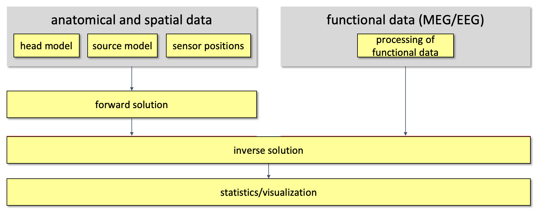
Using this information, source estimation comprises two major steps: (1) Estimation of the EEG potential or MEG field distribution for a known source is referred to as forward modeling. (2) Estimation of the unknown sources corresponding to the measured EEG or MEG is referred to as inverse modeling.

The forward solution can be computed when the head model, the sensor positions and a model for the source are given. For distributed source models and for scanning approaches such as beamforming, the source model consists of a discrete description of the the brain volume or of the cortical sheet in many voxels or vertices. When the forward solution is computed, the lead field matrix (with dimensions Nchan * Nsources) is calculated for each point, taking into account the head model and the sensor positions.

A prerequisite of forward modeling is that the geometrical description of the sensor positions, head model and source model are expressed in the same coordinate system (e.g., CTF, MNI, Talairach) and with the same units (mm, cm, or m). There are different conventions for coordinate systems. The precise coordinate system is not relevant, as long as all data is consistent. Here you can read how the different head and MRI coordinate systems are defined. For most MEG systems, the gradiometers are by default defined relative to head localizer coils or anatomical landmarks, therefore when the anatomical MRI are aligned to the same landmarks, the position of the MEG sensors directly matches the MRI. As EEG data is typically not explicitly aligned relatively to the head, therefore, the EEG electrodes usually have to be explicitly realigned prior to source reconstruction (see also this faq and this example).

Figure 1. Overall outline of the pipeline used for source reconstruction

This tutorial is focusing on how to build the FEM volume conduction model for the head, which is also known as the head model.

A volume conduction model of the head, also known as a head model, is represented in FieldTrip as a MATLAB structure. It describes how the currents flow through the tissue, not where they originate from. In general it consists of a description of the geometry of the tissue(s), a description of the conductivity of the tissue(s), and mathematical parameters that are derived from these. How the mathematical parameters are described depends on the computational solution to the forward problem, either by numerical approximations (e.g., using the boundary element and finite element method, or BEM and FEM), or by exact analytical solutions (e.g., for spherical models).

The more accurate the description of the geometry of the head or the source, the better the quality of the forward model. There are many types of head models which, to various degrees, take the individual anatomy into account. The different head models available in FieldTrip are listed here.

Procedure

Here, we will work towards a volume conduction model of the head based on the Finite Element Method (FEM). The FEM assumes realistic geometrical information about the head, including the skin, skull, csf, gray, and white matter. It can include more tissue types, and in contrast tp the BEM, the geometry of each tissue type can be arbitrary complex.

The procedure starts with classifying each of the voxels in the anatomical MRI as one of the tissue types that we want to model; this is termed segmentation. Following the segmentation, we construct a tetrahedral or hexahedral mesh that describe the different tissue types. Finally, the FEM model will be computed using the conductivities of the corresponding tissue types.

The anatomical MRI of the tutorial data set is available here. Although we did not record EEG in this study, we will nevertheless use it as example MRI to make an BEM volume conduction model for EEG.

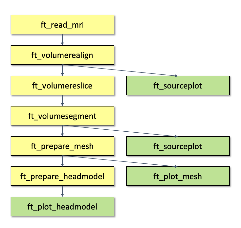
• we read the anatomical data with ft_read_mri
• if needed, we use ft_volumerealign to align the MRI with the desired coordinate system
• if needed, we use ft_volumereslice to flip the volume so that it points up
• we segment the anatomical information into different tissue types with ft_volumesegment
• we make a mesh that describes all tissue types with ft_prepare_mesh
• we create the headmodel with ft_prepare_headmodel

Throughout the process we use ft_sourceplot, ft_plot_mesh and ft_plot_headmodel to check that each of the steps was executed correctly.

Figure; Pipeline for creating a FEM model

Reading in the anatomical data

Before starting with FieldTrip, it is important that you set up your MATLAB path properly.

cd <path_to_fieldtrip>
ft_defaults

Then, you can read in the anatomical MRI data.

mri = ft_read_mri('Subject01.mri');

save mri mri

disp(mri)
          dim: [256 256 256]
      anatomy: [256x256x256 int16]
          hdr: [1x1 struct]
    transform: [4x4 double]
          fid: [1x1 struct]
          unit: 'mm'
      coordsys: 'ctf'

The structure of the mri variable contains the following fields:

• dim gives information on the size (i.e. the number of voxels) of the anatomical volume into each direction
• anatomy is a matrix (with the size and number of dimensions specified in dim) that contains the anatomical information
• hdr contains the detailed header information from the original file, it contents vary, depending on the file format
• transform is a homogenous transformation matrix that allows expressing the voxel positions (in the field anatomy) in a certain coordinate system
• fid is an optional structure with fiducial information, this will in general not be present
• coordsys specifies the coordinate system
• unit specifies the units of distance

You can see that in the data we just read in the coordsys specifies that it is already aligned to the CTF coordinate system. This MRI was not read from the original DICOM images, but was in the past already processed using the CTF MRIConverter tool. We will get back to this in the next section.

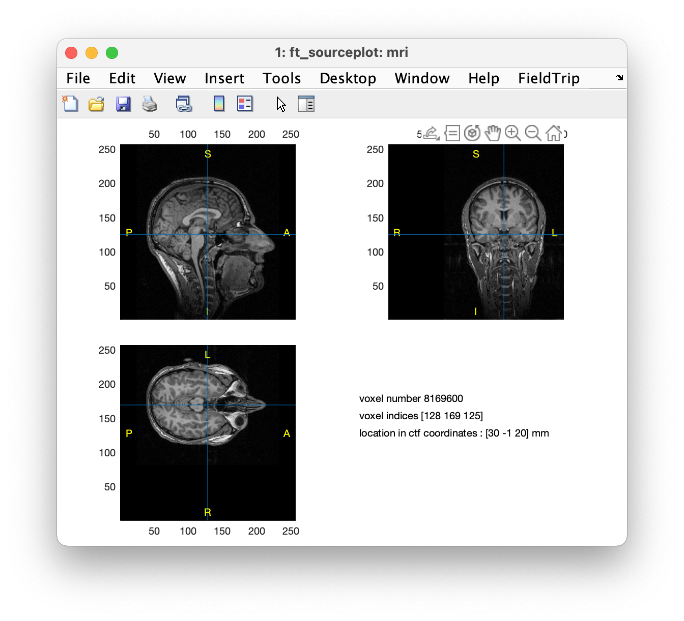
We can check the overall quality of the MRI image using ft_sourceplot, which allows us to browse through the whole volume.

cfg = [];
cfg.method = 'ortho';
ft_sourceplot(cfg, mri)

In case your MRI appears upside down, don’t worry. This is common and we will address it in the next section.

Figure; Using ft_sourceplot to asses the MRI quality

Things to pay attention to when judging the quality of the MRI are

• is the MRI image of good quality overall?
• is the coverage complete, including the tip of the nose, back and top of the head and the ears? Complete coverage is especially important for EEG, as the headmodel includes the scalp.
• is the MRI contrast homogenous over the whole volume? If not, consider ft_volumebiascorrect.
• do you see the fiducials that you expect, such as vitamine-E capsules? In this case there are earmold markers along the ear canals, and a marker behind the right ear (for a left/right check).
• is the part of the MRI outside the head (i.e., the air) uniform and black? If not, you might be able to clean it up with ft_defacevolume.
• are the anatomical landmarks at the expected coordinates? In this case the nasion is at (116,0,0) mm, the left ear at (0,72,0) mm, the right ear at (0,-71,0) mm, in line with the CTF convention. If not, you will have to realign the MRI to the desired coordinate system (see next section).

Align the MRI to the head coordinate system

The EEG head model needs to be expressed in the same coordinate system as the electrodes and the source model. It is not really relevant which specific coordinate system is used, as long as all are consistently aligned.

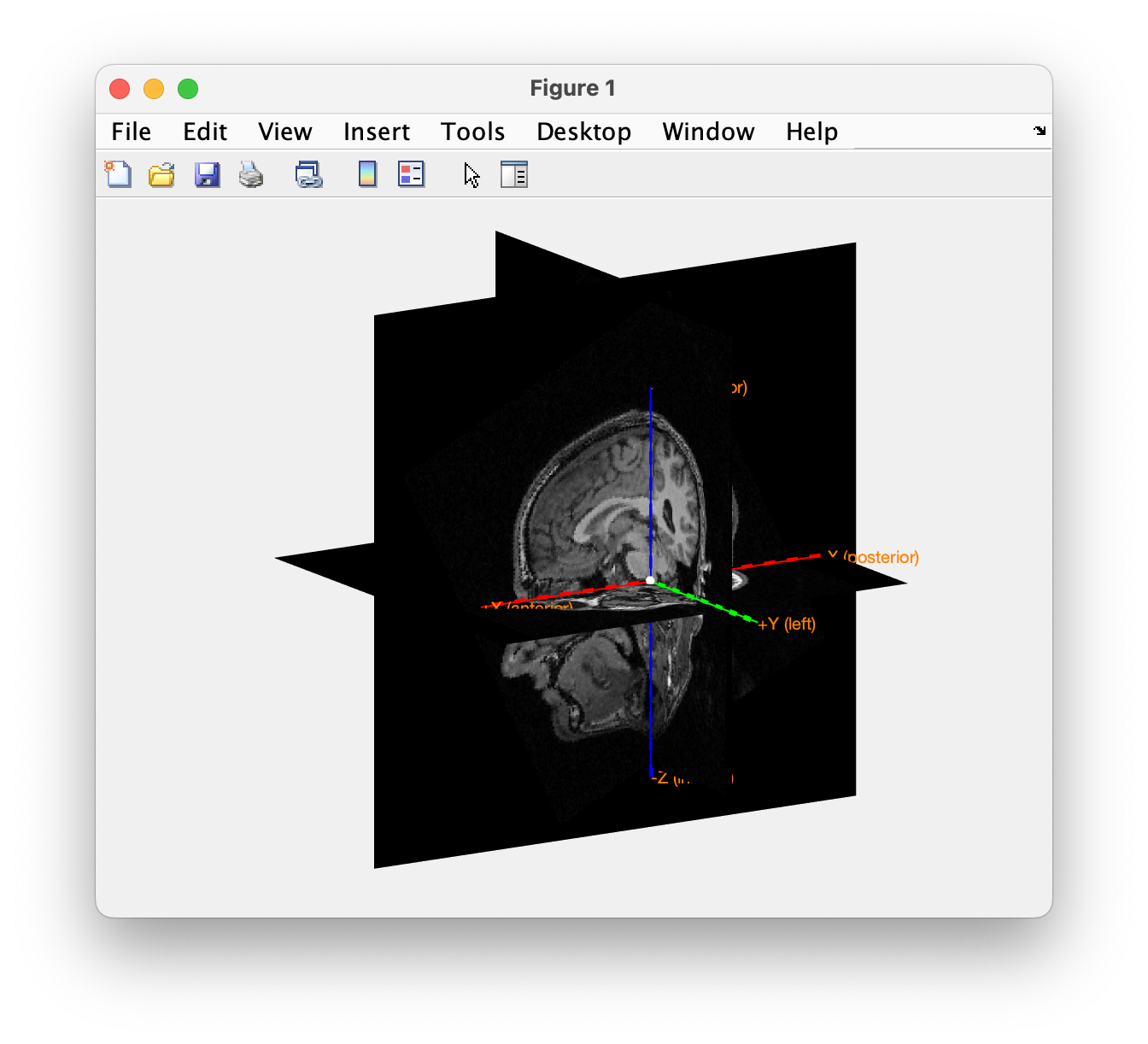
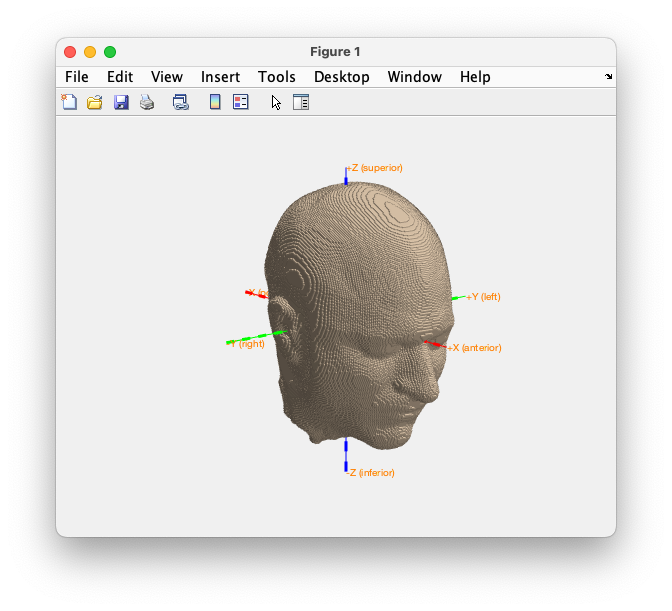
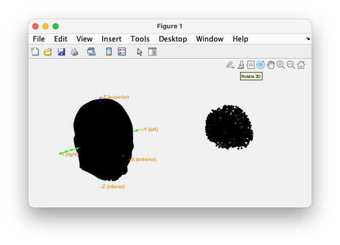
Using ft_sourceplot we can check the orientation of the axes and the position of the origin by looking at the numbers taht are printed on screen. Alternatively, we can make a 3D image with ft_determine_coordsys. In the command window it will print that the positive x-axis is pointing towards “anterior”, the positive y-axis is pointing towards the “left” and the positive z-axis is pointing towards “superior”, in line with the CTF convention. You can also see this in the figure, which has the x-axis (red), y-axis (green) and z-axis (blue) pointing in these three directions of the head. The figure also reveals that the y-axis passes through both ears, consistent with the convention at the Donders Centre for Cognitive Neuroimaging (DCCN).

ft_determine_coordsys(mri)
% rotate the anatomical MRI around and pay attention to the labels along the axes
% press "n" and "return" in the command window

Figure; Determine the coordinate system in which the original MRI is expressed

You might read your anatomical MRI data from DICOM files, from a NIFTI file, or other formats, with data that is possibly defined in a different coordinate system. In that case it may not give information on the coordinate system in which the anatomical data is expressed. You can check and update the coordinate-system with the ft_determine_coordsys function by specifying in which direction eax axis points and where the origin is relative to the head.

In general following the reading of the MRI, we use ft_volumerealign to align the anatomical MRI to the desired coordinate system. For the CTF coordinate system - as for most coordinate systems used in EEG and MEG - you have to specify the anatomical landmarks (LPA, RPA and nasion). Knowing the voxel indices of these landmarks allows the MRI to be translated and rotated such that the axes of the coordinate systems pass through these landmarks. Following the coregistration or realignment of the MRI, the output of any later processing step on the MRI (reslicing, segmentation, mesh, headmodel) will be expressed in the same coordinate system. Once all anatomical processing of the MRI is done, you can also align the electrodes to the same anatomical landmarks and/or you can fit the electrodes interactively on the scalp surface of your head model.

In this specific case the anatomical MRI is already aligned to the CTF coordinate system. Therefore, we do not need to align the anatomical MRI to any other convention. But if needed, we could have used the previous ft_sourceplot step to identify and write down the voxel indices of the nasion, LPA and RPA.

Using the fiducial locations (in voxels) written down in the previous step, we would do

cfg = [];
cfg.method = 'fiducial';
cfg.fiducial.nas = [ 87   60  116];
cfg.fiducial.lpa = [ 29  145  155];
cfg.fiducial.rpa = [144  142  158];
cfg.coordsys = 'ctf'; % the desired coordinate system
mri_realigned = ft_volumerealign(cfg, mri)

save mri_realigned mri_realigned

If we did not pay attention to the anatomical landmarks when looking at ft_sourceplot, we could also use ft_volumerealign to find them.

cfg = [];
cfg.method = 'interactive'
cfg.coordsys = 'ctf'; % the desired coordinate system
mri_realigned = ft_volumerealign(cfg, mri)

Identifying the nasion is easy. However, it is difficult, if not impossible, to visually distinguish the left and right side from the anatomical MRI. That is why at the DCCN (where this scan was made) we always include a vitamine-E capsule at the right side of the head. Sometimes the vitamine-E capsule is taped on the right mastoid, sometimes it is taped into the right earshell of the protective headphones. To determine the rpa in this specific MRI, you first search for the vitamine-E capsule and then search for the fiducial that marks the right ear canal. Once the rpa been determined, you can move on to the lpa. Other labs might use vitamine-E capsules at the anatomical landmarks themselves, or might not use any fiducials, so please update your own coregistration procedure accordingly.

Exercise 1

Reslicing

A common issue with anatomical MRI data is that it is plotted upside down. This is not necessarily a problem for the FEM model that we will make, as we know the position of each MRI voxel relative to the coordinate system, but it is a bit inconvenient in the plotting of MRI slices and quality control later in the pipeline.

The ft_volumereslice function can be used to flip the volume such that the 1st dimension of the three-dimensional mri.anatomy array corresponds approximately with the x-axis of the coordinate system, that the 2nd dimension corresponds approximately to the y-axis, and the 3rd dimension to the z-axis.

Note that the axes of the coordinate system in general will not be exactly aligned with the orientation and direction of the slices of the MRI during acquisition. You can also use ft_volumereslice to properly reslice your anatomical MRI; in that case it will be interpolated onto a regular and isotropic grid in which the volume is aligned with the axes and the size of the voxel is identical in each direction. This is recommended when you use morphological image operations such as imerode and imdilate, which is common for constructing the segmentation that underlies the triangulated surfaces for the boundary element method (BEM).

The following flips the volume such that the anatomical volume approximately aligns with the axes

cfg = [];
cfg.method = 'flip';
mri_resliced = ft_volumereslice(cfg, mri_realigned);

save mri_resliced mri_resliced

If you would want to align it exactly with the axes and/or make the voxels isotropic, you could use the ‘linear’ method in ft_volumereslice.

Following the reslicing, the MRI should be shown with the correct side up, the field-of-view should be symmetric from left to right. If you move along the first axis, you should see that the first voxel index i increase and that the x position increases (idem for j/y and k/z).

cfg = [];
cfg.method = 'ortho';
ft_sourceplot(cfg, mri_resliced)

Figure; The MRI after assigning the desired coordinate system and reslicing

You should check that all parts of the head are present in the resliced images, including the nose, back of the head and the top of the head. If not, you need to redo the reslicing with a slightly modified vield of view.

Segmentation

In this step, the voxels of the anatomical MRI are segmented or classified using ft_volumesegment into the three different tissue types: scalp, skull, csf (cerebro-spinal fluid), gray and white matter. You can read more about how the tissue-types are represented in the output of this function in this FAQ. The resulting segmentation should be a binary representation of the 5 tissue types without overlap, i.e., each voxel belongs to exactly one tissue type.

cfg           = [];
cfg.output    = {'gray', 'white', 'csf', 'skull', 'scalp'};
segmentedmri  = ft_volumesegment(cfg, mri_resliced);

save segmentedmri segmentedmri

 disp(segmentedmri)
           dim: [256 256 256]
     transform: [4x4 double]
      coordsys: 'ctf'
          unit: 'mm'
          gray: [256x256x256 logical]
         white: [256x256x256 logical]
           csf: [256x256x256 logical]
         skull: [256x256x256 logical]
         scalp: [256x256x256 logical]
           cfg: [1x1 struct]

The segmentedmri data structure is similar to the mri data structure, but contains the new fields:

• gray: binary representation of the grey matter, note the difference between UK and US spelling
• white: binary representation of the white matter
• csf: binary representation of the CSF
• skull: binary representation of the skull
• scalp: binary representation of the scalp

The segmentation does not change the coordinate system, nor the size of the voxels or volume. You can see this in the first three fields (dim, transform and coordsys) which are the same as the corresponding fields in the MRI. The field transform aligns the 3D array in gray,, white, csf, skull and scalp to the coordinate system defined in the coordsys field, just like it did for the anatomy field in the anatomical MRI. It is good practice to check at this point in a figure, whether the segmented compartments look as expected.

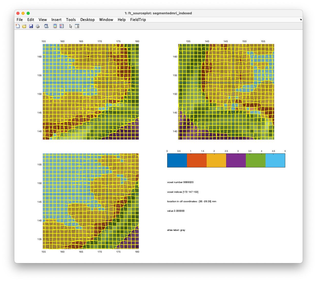
The function ft_sourceplot can be used to plot the segmented tissues. To see all tissues in one image, we use ft_datatype_segmentation to convert the segmentation structure to an indexed representation. Each tissue type has a different value and will be shown by a different color.

% convert from probabilistic/binary into indexed representation
segmentedmri_indexed = ft_datatype_segmentation(segmentedmri, 'segmentationstyle', 'indexed');

% also add the anatomical mri
segmentedmri_indexed.anatomy = mri_resliced.anatomy;

cfg              = [];
cfg.anaparameter = 'anatomy';
cfg.funparameter = 'tissue';
cfg.funcolormap  = lines(6);              % distinct color per tissue + background
cfg.atlas        = segmentedmri_indexed;  % this is just like an anatomical atlas, see https://www.fieldtriptoolbox.org/template/atlas/
cfg.location     = 'center';
ft_sourceplot(cfg, segmentedmri_indexed);

Figure. Binary representations of gray matter, white matter, csf, skull, and scalp

Meshing

The next step is to create a geometrical description of the head by the ft_prepare_mesh function. At the moment FieldTrip-SIMBIO only supports hexahedra. The hexahedral mesh elements consist of 8 vertices at the corners that are connected like cubes. Each hexahedron is assigned to one of the five tissue-types.

To improve how the mesh approximates the head shape, a node-shift can be applied. This shifts vertices at the boundaries in the direction of those hexahedra that represent the minority around it (see figure). The magnitude of the shift is controlled by a shift parameter which can range from 0 (no shift) to 0.3.

cfg        = [];
cfg.shift  = 0.3;
cfg.method = 'hexahedral';
mesh = ft_prepare_mesh(cfg, segmentedmri);

save mesh mesh

disp(mesh)
            pos: [2372249x3 double]
            hex: [2301983x8 double]
         tissue: [2301983x1 double]
    tissuelabel: {'csf'  'gray'  'scalp'  'skull'  'white'}
           unit: 'mm'
       coordsys: 'ctf'
            cfg: [1x1 struct]

The mesh contains the following field

• pos : The position of the vertices.
• hex : Each row defines 8 corners of a hexahedron (row numbers of the pnt field).
• unit: Units in which the vertices are expressed.
• tissue: Each hexahedron (in hex) is indexed with a value from 1…N. These values represent the tissue-types and are assigned to each type according to the order in tissuelabel.
• tissuelabel: Names of tissue-types.

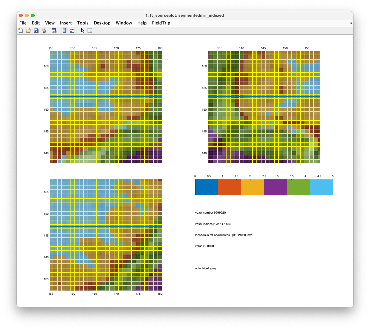
You can plot the anatomical MRI, the segmentation and the hexahedral mesh together in one figure. Note that you will have to zoom in quite a bit to see the individual hexahedral elements, as there are so many.

cfg = [];
cfg.funparameter = 'tissue';
cfg.anaparameter = 'anatomy';
cfg.atlas = segmentedmri_indexed; % this is just like an anatomical atlas, see https://www.fieldtriptoolbox.org/template/atlas/
cfg.funcolormap = lines(6);
cfg.method = 'ortho';
cfg.intersectmesh = mesh;
ft_sourceplot(cfg, segmentedmri_indexed)

Figure. Comparison of a shifted mesh (upper) and unshifted mesh (lower).

The visualization can also be done using Seg3D or ParaView. With Seg3D you can make modifications to the segmentation.

Compute the FEM head model

Now that gray matter, white matter, csf, skull and skin has been modeled as a mesh, we will create the volume conduction model. We will specify cfg.method='simbio' in ft_prepare_headmodel. This methods also requires to specify the conductivities for each tissue-types. The headmodel can also be downloaded from our download server.

cfg        = [];
cfg.method = 'simbio';
cfg.conductivity = [1.79 0.33 0.43 0.01 0.14];   % the order follows mesh.tissuelabel, which is 'csf', 'gray', 'scalp', 'skull', 'white'
headmodel  = ft_prepare_headmodel(cfg, mesh);

save headmodel headmodel

disp(headmodel)
            pos: [2372249x3 double]
            hex: [2301983x8 double]
         tissue: [2301983x1 double]
           cond: [1.79 0.33 0.43 0.01 0.14]
    tissuelabel: {'csf'  'gray'  'scalp'  'skull'  'white'}
          stiff: [2372249x2372249 double]
           type: 'simbio'
           unit: 'mm'
            cfg: [1x1 struct]

The headmodel data structure contains the same information in the pos, hex, tissue and tissulabel fields than the mesh we created earlier. And it has also new fields:

• cond: conductivity of each tissue-type (in order of tissuelabel)
• stiff: matrix
• type: describes the method that was used to create the headmodel.

Note that the unit of measurement used in the geometrical description of headmodel is in ‘mm’. The EEG sensors should be also defined in ‘mm’. The units of all type of geometrical information should be the same when a leadfield is computed for source reconstruction.

Visualization

The hexahedral mesh is a geometrical description of the head. It is built up from hexahedra. For visualization, it is possible to use the ft_plot_mesh function which is generally used for plotting any type of meshes in FieldTrip. Because of the large number of points in a mesh, it is advised to use the ‘surfaceonly’ option. In this case, the function will plot hexagonal surfaces of those hexahedra which create the outside surface of the head.

ft_plot_mesh(mesh, 'edgecolor','none', 'facecolor', 'skin', 'facealpha', 0.7);
ft_plot_axes(mesh)
alpha 1
material default
camlight

Figure. Plot of the FEM mesh

This only shows the outside of the scalp. To see the other tissues, you can split the mesh into the different tissue types and make one mesh for each.

% make a copy for each tissue type
% after splitting we don't need the tissue and tissuelabel any more
mesh_csf   = rmfield(mesh, {'tissue', 'tissuelabel'});
mesh_gray  = rmfield(mesh, {'tissue', 'tissuelabel'});
mesh_scalp = rmfield(mesh, {'tissue', 'tissuelabel'});
mesh_skull = rmfield(mesh, {'tissue', 'tissuelabel'});
mesh_white = rmfield(mesh, {'tissue', 'tissuelabel'});

% only keep the hexahedra for the corresponding tissue type
mesh_csf.hex   = mesh.hex(mesh.tissue==1,:);
mesh_gray.hex  = mesh.hex(mesh.tissue==2,:);
mesh_scalp.hex = mesh.hex(mesh.tissue==3,:);
mesh_skull.hex = mesh.hex(mesh.tissue==4,:);
mesh_white.hex = mesh.hex(mesh.tissue==5,:);

Alternatively, you can write the mesh to a file on disk with ft_write_headshape and use ParaView for visualization.

Align EEG electrodes

The procedure to align the electrodes is basically the same as for a BEM head model which you can read in much more detail here. Very shortly: you can do the following to align it to the FEM mesh.

% you may need to specify the full path to the file
elec = ft_read_sens('standard_1020.elc');

disp(elec)
    chanpos: [97x3 double]
   chantype: {97x1 cell}
   chanunit: {97x1 cell}
    elecpos: [97x3 double]
      label: {97x1 cell}
       type: 'eeg1010'
       unit: 'mm'

cfg = [];
cfg.method = 'interactive';
cfg.headshape = mesh; % we can specify the hexahedral FEM mesh as the headshape
elec_realigned = ft_electroderealign(cfg, elec)

save elec_realigned elec_realigned

Since rotations and translations do not “commute”, i.e. the order in which you execute the rotation matters, it can be confusing to specify all rotations and translations in one go. Instead, you can use the “apply” button to do the transformations stepwise.

In this situation we need

• rotate -90 around z; apply
• translate 35 along x and 35 along z; apply
• scale 0.98 along x, 0.90 along y, and 0.80 along z; apply
• translate 25 along z; apply
• rotate 11 degrees around y, translate -5 along x; apply
• quit

Figure; Use the GUI to align the electrodes.

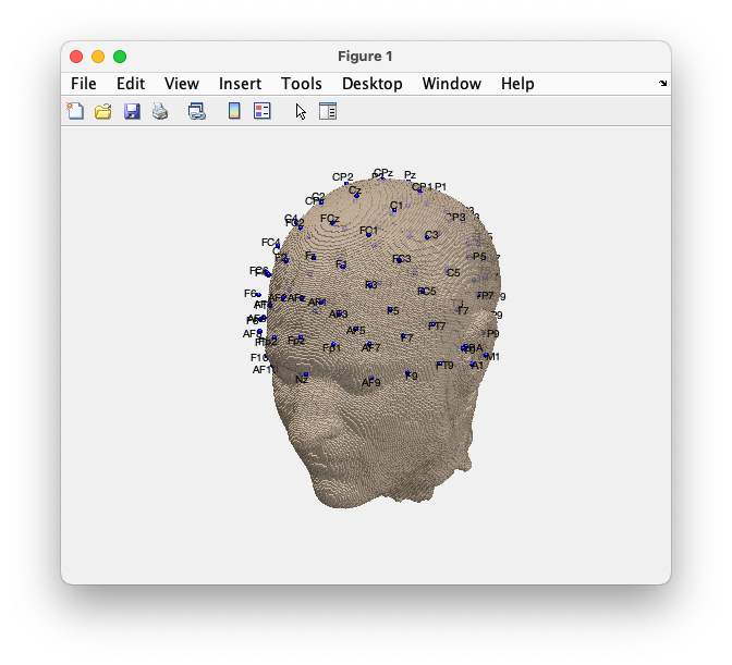
Using a final plot that includes the electrode labels, we can check that it all matches.

figure
ft_plot_headmodel(headmodel, 'facecolor', 'skin', 'facealpha', 0.7);
hold on
ft_plot_sens(elec_realigned, 'elecshape', 'sphere', 'label', 'on');
camlight

Figure; Realigned electrodes plotted together with the scalp surface.

This electrode structure can be used later when the leadfield is computed with ft_prepare_leadfield and ft_sourceanalysis, or with ft_dipolefitting. During the computation of the leadfield, the electrodes will be projected exactly onto the scalp surface, so don’t worry if the fit is not yet 100% perfect.

Construct source model

With single-shell and BEM volume conduction models you can place the dipoles of the source model anywhere in the brain compartment. With more detailed FEM models, you want the dipoles only in the grey matter. Furthermore, the FEM computations will be more accurate if the dipoles are placed at the centroids of the volume elements.

The following starts with a 8 mm regular grid. The dipole positions are subsequently moved to the nearest centroid.

cfg = [];
cfg.method = 'basedonresolution';
cfg.resolution = 8; % in mm
cfg.unit = 'mm';
cfg.headmodel = mesh;
cfg.headmodel.type = 'simbio';
cfg.movetocentroids = 'yes';
sourcemodel = ft_prepare_sourcemodel(cfg)

save sourcemodel sourcemodel

We can plot the complete sourcemodel and compare it to only the sources inside the grey matter. This makes use of the MATLAB linkprop command to keep the two subplots in sync.

figure
ax1 = subplot(1,2,1); ft_plot_mesh(sourcemodel); ft_plot_axes(sourcemodel)
ax2 = subplot(1,2,2); ft_plot_mesh(sourcemodel.pos(sourcemodel.inside,:))

hlink = linkprop([ax1, ax2], {'CameraPosition', 'CameraUpVector', 'xLim', 'YLim', 'ZLim'});
rotate3d on

Figure; All source positions (left) and those inside the grey matter (right).

There are many dipoles at positions where we will not compute the leadfields anyway, such as the skull and lower parts of the head. We can prune the sourcemodel and select only the dipoles inside grey matter.

sourcemodel.pos    = sourcemodel.pos(sourcemodel.inside,:)
sourcemodel.tissue = sourcemodel.tissue(sourcemodel.inside,:); % also update the tissue indices
sourcemodel.inside = sourcemodel.inside(sourcemodel.inside,:); % and update the inside vector itself

The construction of the sourcemodel above takes quite some time as many dipoles need to be compared with many centroids. We can speed it up by starting with a smaller regular grid of dipoles by explicitly specifying the initial regular grid. This requires knowing the (approximate) boundaries of the brain.

cfg = [];
cfg.method = 'basedongrid';
cfg.xgrid = -80:8:120;  % specified in multiples of 8, so that [0 0 0] is part of the grid
cfg.ygrid = -80:8:80;
cfg.zgrid = -24:8:120;
cfg.unit = 'mm';
cfg.headmodel = mesh;
cfg.headmodel.type = 'simbio';
cfg.movetocentroids = 'yes';
sourcemodel = ft_prepare_sourcemodel(cfg)

Summary and suggested further reading

This tutorial explained how to build a volume conduction model of the head using a single subject anatomical MRI and a finite element method (FEM) using the FieldTrip-SIMBIO pipeline.

You can read more about specific source reconstruction methods in the Localizing oscillatory sources using beamformer techniques and in the Source reconstruction of event-related fields using minimum-norm estimate tutorials.

See also these frequently asked questions

• Can I do combined EEG and MEG source reconstruction?
• How is the segmentation defined?
• How to coregister an anatomical MRI with the gradiometer or electrode positions?

See also these examples

• Combined EEG and MEG source reconstruction
• Compute forward simulated data using ft_dipolesimulation
• Compute forward simulated data with the low-level ft_compute_leadfield
• Align EEG electrode positions to BEM headmodel
• Compute EEG leadfields using a FEM headmodel
• Testing BEM created EEG lead fields