Using a MEG phantom for validation and OPM calibration

Introduction

Magnetoencephalography (MEG) systems need to be validated, calibrated, and their sensors precisely localized before they can be used for recording and especially source-reconstructing brain activity. Phantoms — devices with known, controllable magnetic field sources at precisely known positions — play an essential role in all three of these tasks.

Conventional SQUID-based MEG systems have fixed sensor arrays inside a cryogenic dewar with liquid helium, and their sensor positions are determined once during installation and remain stable. Optically Pumped Magnetometer (OPM) systems, by contrast, use individual sensors that can be flexibly placed on the head, often in 3D-printed helmets. For OPMs, the sensor positions and orientations must be determined for each recording session, making phantom-based validation and calibration even more important.

This tutorial demonstrates three use cases for a spherical MEG phantom equipped with 24 magnetic dipole coils:

1. System validation — testing whether an MEG system correctly localizes known magnetic sources, for comparing SQUID and OPM systems.
2. Channel ampitude calibration — determining the sensitivity of each MEG sensor using the known coil positions.
3. MEG sensor localization — using the phantom to establish the geometry of an OPM sensor array by fitting dipoles to the known coil positions.

Background

Why use phantoms?

MEG phantoms serve three main purposes:

• System acceptance and quality assurance: When a new MEG system is installed, or after maintenance, a phantom measurement verifies that the system is functioning correctly. By comparing the estimated dipole positions and moments with the known ground truth, you can quantify the localization accuracy of the system.
• Sensor calibration: For source reconstruction with MEG systems, the exact position and orientation of each sensor must be known. A phantom with a sufficient number of coils at known positions provides reference signals that can be used to determine or verify the sensor geometry.
• Algorithm development and validation: When developing new analysis methods (e.g., denoising, beamforming, minimum-norm estimation, or dipole fitting), phantoms provide ground-truth data with known source configurations, enabling objective evaluation of the method’s performance.

Types of MEG phantoms

Several types of MEG phantoms exist, each suited to different purposes:

• Current dipole phantoms consist of a conducting sphere (filled with a saline solution) with an embedded current source and sink that approximates an equivalent current dipole. The dipole position can sometimes be adjusted. These phantoms generate weak, brain-like magnetic (or electric) signals and are well-suited for testing the end-to-end performance of an MEG system, including the volume conduction model. The CTF commercial phantom is of this type. The localization accuracy achievable with current dipole phantoms has been studied extensively, typically yielding errors in the range of 1-5 mm for SQUID systems (Leahy et al., 1998).

• Head-shaped phantoms are also filled with a saline solution or a conductive gel, but also aim to replicate the geometry and the electromagnetic properties of the human head. These are required for EEG where the volume conduction of skull and skin is crucial. The combined EEG/MEG phantom described by Leahy et al. (1998) is of this type, and Cao et al. (2023) describe a realistic three-layer head phantom (brain, skull, scalp) designed specifically for OPM-based MEG.

• Dry current dipole phantoms use triangular wire coils to generate magnetic fields that approximate those of equivalent current dipoles (ECDs) in a spherical volume conductor. They do not require a conducting medium and can be precisely manufactured using PCBs or 3D printing. The positions of the wires is well known from the design or can be measured with high precision, providing accurate ground truth. The Neuromag/Elekta/MEGIN commercial phantom and the dry phantom described by Oyama et al. (2015) are of this type.

• Magnetic dipole coil arrays are designed specifically for sensor calibration. They consist of multiple coils arranged on a spherical bobbin, with coil orientations chosen to span a wide range of directions. The spherical coil array described by Adachi et al. (2023) uses 16 coils on a 150 mm diameter sphere based on icosahedral symmetry, and was shown to improve calibration accuracy compared to conventional multi-axis coil bobbin arrays. The HALO described by Hill et al. (2025) is a circular printed circuit board with 16 independently controllable dipolar coils mounted above the OPM helmet, and provides sensor locations within 2 mm of the ground truth.

The dataset used in this tutorial

The dataset used in this tutorial consists of recordings with a 275-channel CTF SQUID system and a 32-sensor/64-channel FieldLine OPM system.

The phantom used in this tutorial is a 120 mm radius sphere with 32 vertices, 24 of which are fitted with radially oriented magnetic dipole coils. These coils are similar to the head localization coils (HLC, also known as HPI coils) that are conventionally placed on anatomical landmarks (the nasion and ears) to determine the position of the head in a whole-head sensor array. The 24 coils are driven by an Arduino Uno-based 24-channel current driver with sinusoidal currents at unique frequencies. The design of both the phantom and current driver are open hardware, allowing you to construct your own, and you can find more details on the open hardware page.

The 24 coils are arranged to provide good angular coverage of the sphere, ensuring that magnetic fields can be generated in many different directions. This is important for calibration, where the goal is to determine the position, orientation, and sensitivity of each sensor by fitting the measured fields to a model with known source positions.

The phantom is placed inside the MEG sensor array (in the helmet for OPM systems, or in the dewar opening for SQUID systems). The recording is typically 1-2 minutes long, during which all coils are active simultaneously at different frequencies. This allows the contribution of each coil to be isolated by bandpass filtering around its drive frequency.

The data used in this tutorial is available from our download server

Procedure

This tutorial covers the following steps:

• Using ft_preprocessing to load and preprocess phantom data recorded with a SQUID or OPM system
• Using ft_freqanalysis to compute and visualize the power spectrum to verify that all coils are active
• Estimating the topographies using ft_componentanalysis
• Using ft_dipolefitting to determine the positions of the phantom coils from the MEG data

Following the estimation of the magnetic dipole positions for all coils, we validate the estimated coil positions with the known ground truth and we evaluate the localization accuracy. Furthermore, we use the known coil positions for sensor gain calibration and for OPM sensor localization.

System validation and quality assurance

The most straightforward use of a phantom is to verify that an MEG system correctly localizes known magnetic sources. This is done by recording data with the phantom inside the sensor array, fitting dipoles to the recorded signals, and comparing the estimated dipole positions with the known dipole coil positions.

Recording protocol

The phantom is placed inside the MEG sensor array (in the helmet for OPM systems, or in the dewar opening for SQUID systems). The 120 mm diameter spherical phantom is sized to fit inside both an adult-size and infant-size OPM helmet. When placing the phantom, we position it so that as many coils as possible are within the sensor array’s coverage area. For this specific spherical phantom the coils 2, 12, and 22 are on the “front” (indicated with a black piece of tape) and should be more or less in the middle towards the opening of the face, so that the lowest coils 23 and 24 are more or less symmetric at the back in the “neck”. Furthermore we ensure that the phantom is stable and does not move during the recording.

Each of the 24 coils is driven sequentially with a sinusoidal current at a unique frequency. In this case the coils were driven at frequencies from 10 Hz up to 17.667 Hz, with steps of 1/3 Hz. This ensures that that each coil’s signal is spectrally separated from all others and that potential harmonics due to non-ideal sinusoidal wave shapes don’t influence the estimates.

The recording is typically 1-2 minutes long, during which all coils are active simultaneously. This allows the contribution of each coil to be isolated by bandpass filtering around its drive frequency.

Read and preprocess the data

%% read the raw data
cfg = [];
cfg.dataset = 'phantom_3031000.01_20260721_01.ds';
cfg.continuous = 'yes';
cfg.channel = 'M*'; % only MEG channels
cfg.coilaccuracy = 2; % use the most accurate model for the MEG gradiometers
data_all = ft_preprocessing(cfg);

% for all subsequent calibrations to be consistent, we have to work with SI units
data_all.grad = ft_convert_units(data_all.grad, 'm');

%% select a clean segment, avoid edges where coils may not be fully active
cfg         = [];
cfg.latency = [0 100]; % seconds, the last part of the data is not valid
data        = ft_selectdata(cfg, data_all);

Visualize the raw data

Before computing the power spectrum, it is good practice to visually inspect the raw data using ft_databrowser. This allows you to identify any obvious artifacts, check that the coil signals are present, and get a feel for the data quality.

cfg = [];
cfg.channel = 'MRC*';
cfg.ylim = [-1 +1] * 0.2e-12;
cfg.layout = 'CTF275_helmet.mat';
cfg.preproc.demean = 'yes';
cfg.preproc.lpfilter = 'yes';
cfg.preproc.lpfreq = 50;
cfg.preproc.hpfilter = 'yes';
cfg.preproc.hpfreq = 1;
cfg.blocksize = 10;
ft_databrowser(cfg, data)

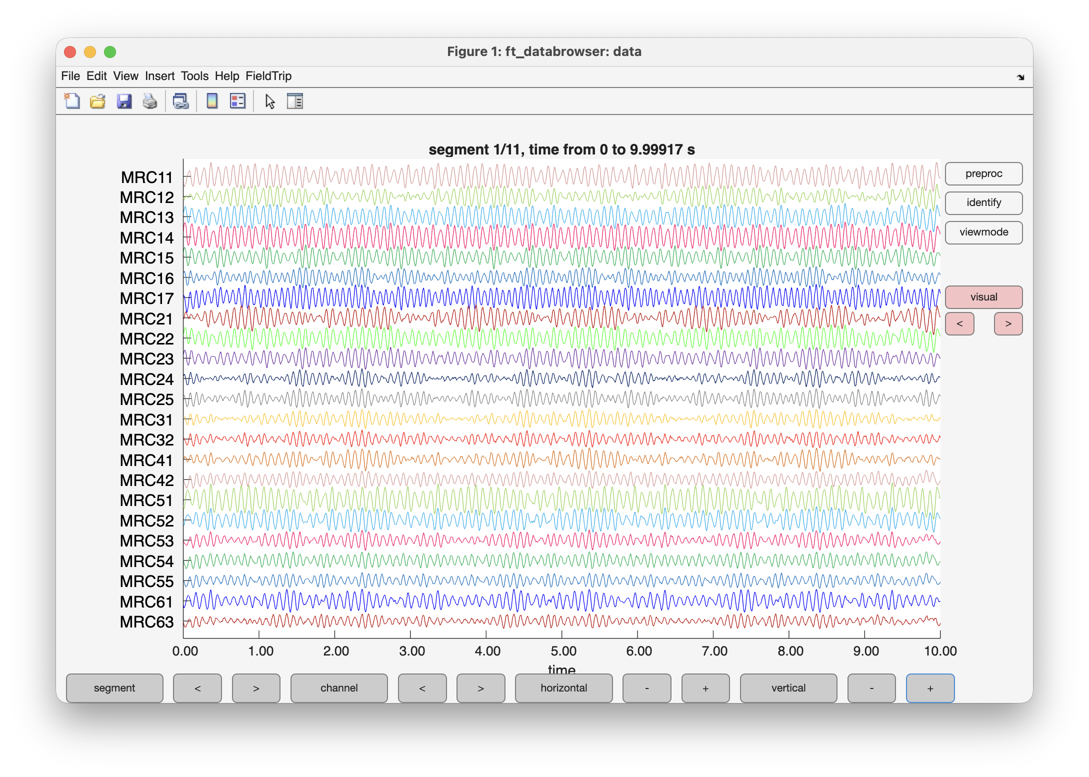
The cfg.preproc options apply a real-time filter while browsing: the high-pass filter at 1 Hz removes slow drifts, the low-pass filter at 50 Hz removes high-frequency noise, and demean = 'yes' removes the DC offset from each channel. This filtering is only applied in the display and does not modify the underlying data.

Visualize the power spectrum

To verify that all 24 coils are active and producing signals at their expected frequencies, we compute and plot the power spectrum. The different coils are simultaneously operated at frequencies from 10 to 17.667 Hz, with 1/3 Hz difference between subsequent coils. That means that the spectral estimation needs to estimate/separate frequencies at integer multiples of 1/3 Hz. Hence we need to segment the data in windows that are 3 seconds long (since that gives a 1/3 Hz frequency resolution), or an integer multiple of that. To properly identify the peaks (and to have throughs in between) we segment the data into 9-second windows with 50% overlap.

cfg = [];
cfg.length = 9;
cfg.overlap = 0.5;
data_segmented = ft_redefinetrial(cfg, data);

cfg = [];
cfg.method = 'mtmfft';
cfg.taper = 'boxcar';
cfg.channel = 'M*';
cfg.foilim = [1 30];
freq = ft_freqanalysis(cfg, data_segmented);

figure;
plot(freq.freq, log10(mean(freq.powspctrm)));
xlabel('frequency (Hz)');
ylabel('log_10 power');
title('phantom power spectrum');

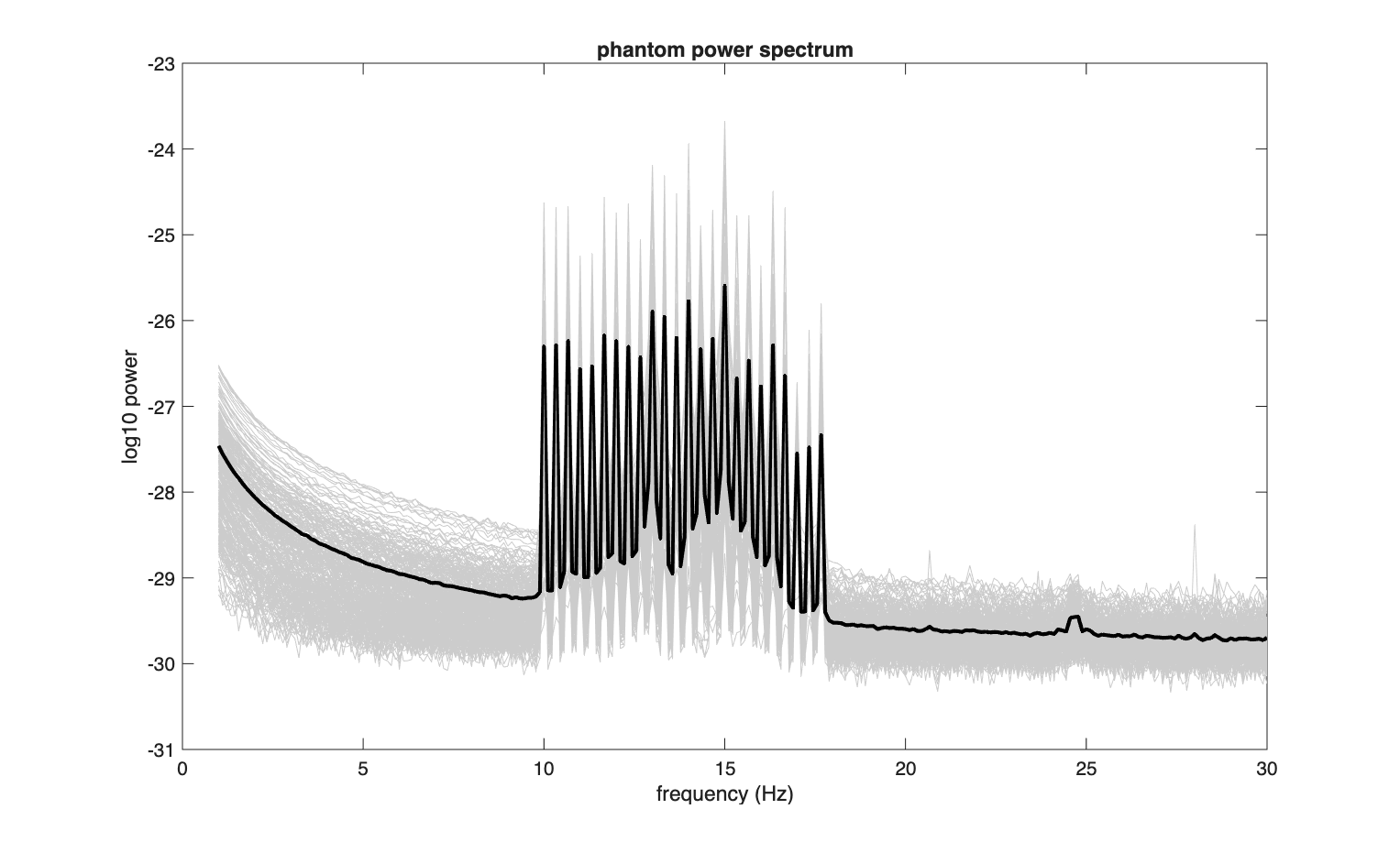
You should see 24 distinct spectral peaks, one for each coil. If any peaks are missing or have unusually low amplitude, the corresponding coil or driver channel may be malfunctioning.

Bandpass filter and estimate topographies

%% define the coil frequencies (one per coil)
coilfreq = 10 + (0:23)/3;

for i=1:24
    cfg = [];
    cfg.bpfilter = 'yes';
    cfg.bpfiltord = 3;
    cfg.bpfreq = [coilfreq(i)-0.1 coilfreq(i)+0.1];
    data_filt{i} = ft_preprocessing(cfg, data);

    cfg = [];
    cfg.method = 'pca';
    cfg.numcomponent = 1;
    cfg.updatesens = 'no';
    pca{i} = ft_componentanalysis(cfg, data_filt{i});
end

The principal component analysis (PCA) decomposes the spatial pattern of the bandpass-filtered data into orthogonal spatial components, ordered by the amount of variance they explain. Because PCA does not know the physical direction of the magnetic field, the sign (polarity) of each component is arbitrary: the same spatial pattern can be represented with either a positive or negative sign. This means that some of the PCA topographies may have their polarity flipped compared to others, which would make it harder to visually compare them.

To ensure a consistent sign convention, we flip the polarity of any component whose maximum absolute value is negative, so that the dominant channel always has a positive weight. The following code plots all 24 topographies in a 3x8 grid after normalizing the sign.

figure

pca = cell(1,24);
for i=1:24

    [m, j] = max(abs(pca{i}.topo));
    if pca{i}.topo(j)<0
        fprintf('flipping pca polarity %d\n', j);
        pca{i}.topo     = -1 * pca{i}.topo;
        pca{i}.trial{1} = -1 * pca{i}.trial{1}; 
    end

    cfg = [];
    cfg.layout = 'CTF275_helmet.mat';
    cfg.zlim = [-0.5 0.5];
    cfg.figure = subplot(3, 8, i); ft_topoplotIC(cfg, pca{i});
end

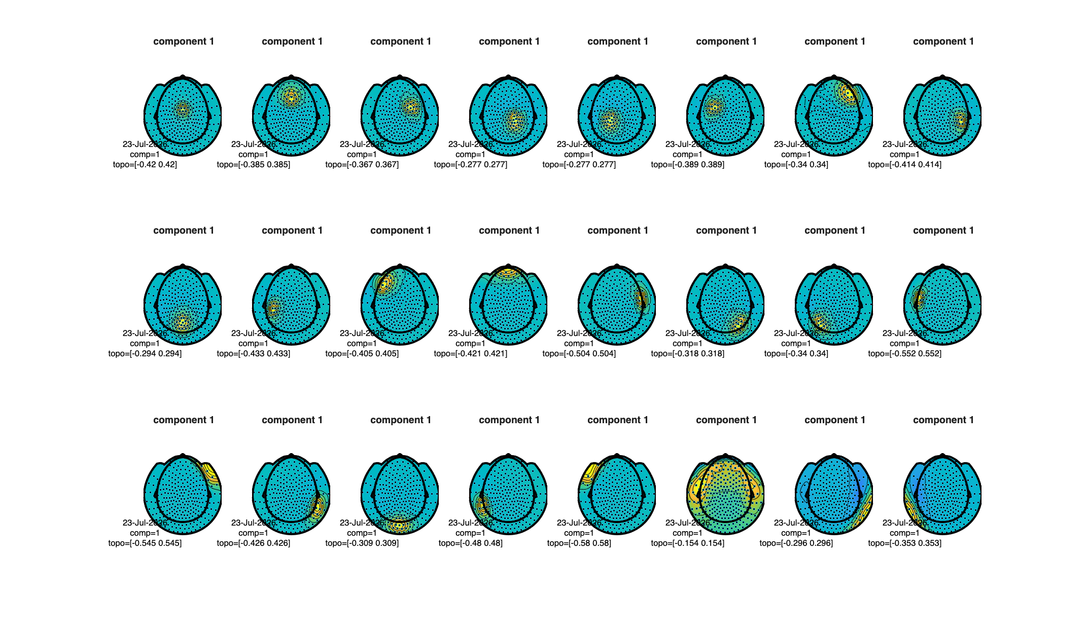
Each subplot shows the spatial topography of one coil’s signal. The topography should look like a focal pattern with a clear peak near the location of the corresponding phantom coil. The focal pattern is characteristic of a magnetic dipole: a region of strong positive field surrounded by weaker negative field (or vice versa, after the sign normalization).

We can also look at the timecourse of the PCA components to check whether they have been properly spatio-temporally separated from the others. As before, you can use your mouse to select a segment of the data and right-click to show the FFT of that segment.

cfg = [];
cfg.viewmode = 'vertical';
cfg.blocksize = 30;
cfg.ylim = [-1 1]*1e-11;
ft_databrowser(cfg, pca{1});

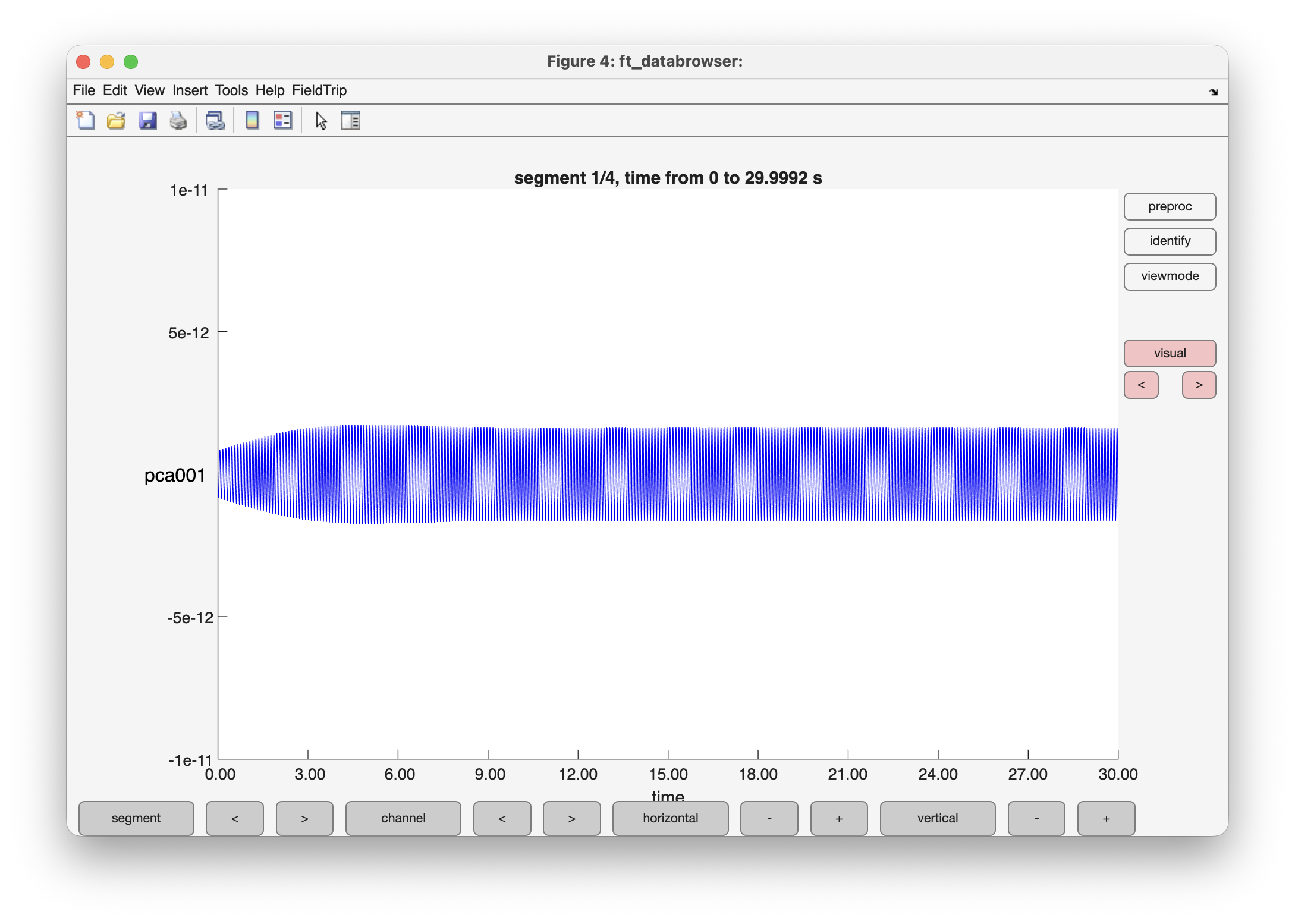
Since the data was bandpass filtered around a single coil frequency, the timecourse of the first PCA component should look like a clean sinusoidal oscillation at that frequency. If the timecourse shows a mixture of different frequencies, it means the bandpass filter was not sufficiently selective or that the coil signals are not well separated in frequency. At the start and end of the data segment there may be edge artifacts from the bandpass filter (the filter needs some time to “ramp up” at the beginning and “ramp down” at the end). These edge artifacts do not affect the PCA topography, because the topography is determined by the spatial pattern across channels, not by the temporal shape of the signal.

Each PCA component is separated in its spatial topography and its timecourse. The topographies are by default normalized, whereas the component timecourse represents the scaling of the actual signal; in this case it represents field strength and is expressed in T. We will ignore the timeseries from now on and continue only with the topographies. To maintain a correct sense of physical units, we will scale the topographies and timeseries such that the timeseries has a standard deviation of 1.

for i=1:24
    scale = std(pca{i}.trial{1});
    pca{i}.trial{1}  = pca{i}.trial{1}  / scale;
    pca{i}.topo(:,1) = pca{i}.topo(:,1) * scale;
end

After this step, the timeseries are normalized, and the topographies represents field strength and are expressed in T.

Fit dipoles for each coil

The procedure for fitting a dipole to each coil is the same as the procedure used for fitting HPI coils in the coregistration of OPM data tutorial. For each coil frequency, a dipole is fitted to the spatial topography of the first principal component.

% crate a sphere that fits nicely inside the helmet to restrict the grid search
fake_headmodel.r = 0.10;
fake_headmodel.o = [0.00 0 0.06];
fake_headmodel.unit = 'm';

% the radius and origin of the sphere needs to be updated until you are happy with how the sphere fits inside the helmet
figure
ft_plot_sens(data.grad, 'chantype', 'meggrad');
ft_plot_headmodel(fake_headmodel, 'facecolor', 'lightskyblue'); % see https://www.rapidtables.com/web/color/html-color-codes.html
ft_headlight

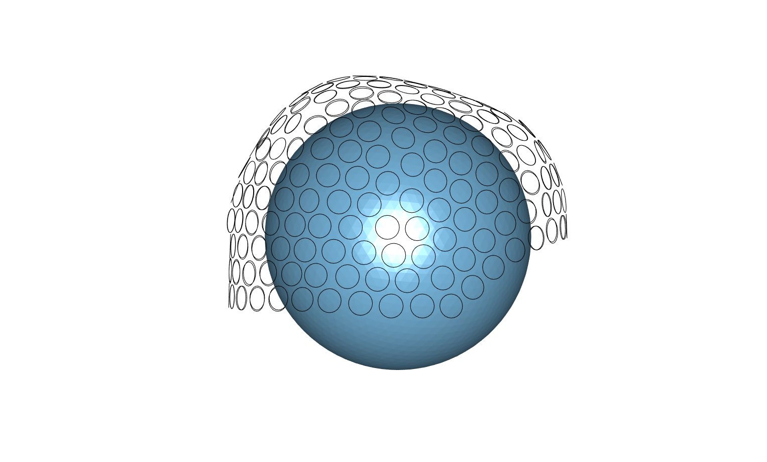
% this starts with a rather wide grid of dipoles at 1cm resolution
% of which only the ones inside the fake headmodel will be used
cfg = [];
cfg.method = 'basedongrid';
cfg.xgrid = -0.20:0.01:0.20;
cfg.ygrid = -0.20:0.01:0.20;
cfg.zgrid = -0.04:0.01:0.20;
cfg.grad = grad;
cfg.headmodel = fake_headmodel;
sourcemodel = ft_prepare_sourcemodel(cfg);

figure
ft_plot_sens(grad, 'axes', 'on', 'chantype', 'meggrad')
ft_plot_mesh(sourcemodel.pos(sourcemodel.inside,:))

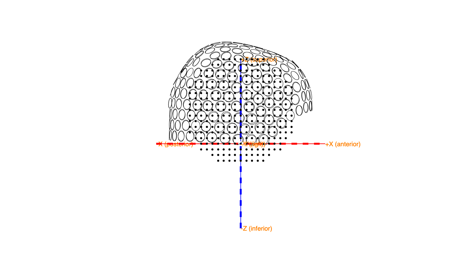
For each of the PCA copmponents we di a grid search over all dipole positions within the sphere, which is then followed by a non-linear optimization during which the dipole drifts from the optimal 1 cm grid location to the actual location where the topographic error is minimal.

% the real heamodel for the magnetic dipole forward computations is an infinite empty space
real_headmodel = [];
real_headmodel.type = 'infinite';
real_headmodel.unit = 'm';

dip = cell(1,24);
for i=1:24
    cfg = [];
    cfg.gridsearch = 'yes';
    cfg.nonlinear = 'yes';
    cfg.sourcemodel = sourcemodel;
    cfg.headmodel = real_headmodel;
    cfg.component = 1;
    cfg.channel = 'M*';
    cfg.grad = grad;
    dip{i} = ft_dipolefitting(cfg, pca{i});

    % store the dipole positions and orientations
    est_pos(i,:) = dip{i}.dip.pos;
    est_ori(i,:) = dip{i}.dip.mom / norm(dip{i}.dip.mom);
end

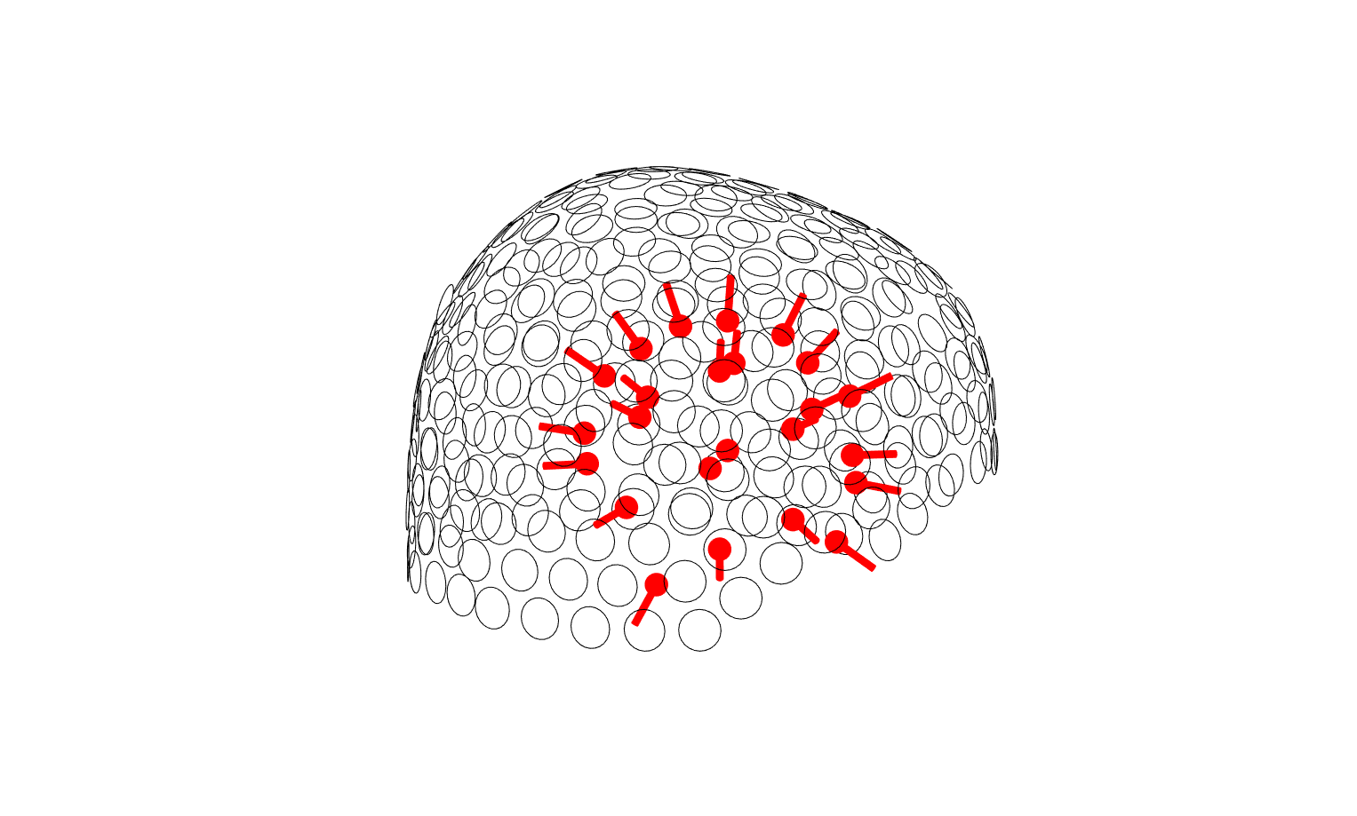
After fitting all dipoles, we want to see where they end up. The dipole orientation can be randomly flipped 180 degrees. By checking the dot product with the position from the center of the helmet we ensure that all dipoles point outward.

figure
ft_plot_sens(grad, 'chantype', 'meggrad')

flip = ones(1,24);
for i=1:24
    pos = est_pos(i,:);
    ori = est_ori(i,:);

    if dot(ori,  pos-fake_headmodel.o)<0
        fprintf('flipping dipole orientation %d\n', i);
        ori     = -ori;
        flip(i) = -1; % remember which ones to flip
      end

    ft_plot_dipole(pos, ori, 'diameter', 0.01, 'length', 0.02)
end

Compare estimated positions with ground truth

The known coil positions from the CAD model serve as ground truth. The localization error for each coil is the distance between the estimated and true position. However, the CAD model is expressed in its own coordinate system, and the fitted dipoles are expressed in the coordinate system of the MEG sensor definition (the “grad” structure). Furthermore, depending how the phantom sphere was placed in the helmet, the dipole positions would also be different. Hence there is an unknown translation and rotation between the two. We can use ft_electroderealign to automatically fit the position of the vertices of the CAD model to the dipole positions

Align the CAD model with the fitted dipole positions

The ft_electroderealign function can map a template description of electrode positions to a subset of electrodes. Using a Polhemus to localize all electrode positions of a high-density (64 or more) EEG cap can be a lot of work; this functionality allows you to localize a subset of electrodes, for example only a few key electrode locations around the head (like FPz, Cz, Oz, T7 and T8) or the 21 electrodes from the 10-20 system, and match those to the corresponding template positions. Based on the spatial transformation of the template subset to the measured locations, all template electrode positions can be spatially transformed to the actually measured coordinate system.

Here we can use the same functionality to determine the spatial transformation from the (arbitrary) coordinate system in which the CAD design was expressed, to the MEG helmet coordinate system in which the dipole positions were fitted. We get the coil positions from the CAD model sphere with 60 mm radius (or 120 mm diameter) that was triangulated using 32 vertices. The 3-D printed coils themselves are 3.2 mm thick, which means that the position of the coils is 1.6 mm outward from the vertex positions. Hence we shift the vertex positions outward by dividing the positions by 60 and multiplying by 60+1.6.

load cad_mesh.mat
cad_mesh = ft_convert_units(cad_mesh, 'm');
cad_mesh.pos = cad_mesh.pos * (60+1.6)/60;

% construct a set of EEG electrodes, one for each of the 24 vertices
model = [];
for i=1:24
    model.elecpos(i,:) = cad_mesh.pos(i,:);
    model.elecori(i,:) = cad_mesh.pos(i,:) / norm(cad_mesh.pos(i,:));
    model.label{i}     = num2str(i);
end
% coil 23 and 24 are not on vertex 23 and 24
model.elecpos(23,:) = cad_mesh.pos(28,:); % coil 23 is placed on vertex 28
model.elecpos(24,:) = cad_mesh.pos(30,:); % coil 24 is placed on vertex 30
model.unit = 'm';

figure
ft_plot_mesh(cad_mesh, 'facecolor', 'beige'); % see https://www.rapidtables.com/web/color/html-color-codes.html
ft_plot_sens(model, 'elec', true, 'axes', true, 'label', 'label', 'elecsize', 0.01, 'elecshape', 'disc')
view(125, 30)

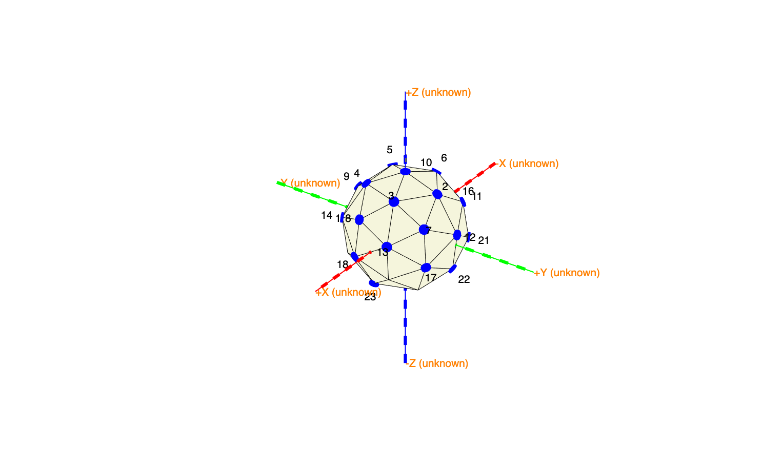
The phantom is not symmetric along the front-back direction and the coils numbered 2, 12, and 22 are the “front” of the phantom and should be towards the usual nose direction, which is +x for the CTF system

cad_mesh = ft_transform_geometry([0 0 -90], cad_mesh, 'rotate');
model    = ft_transform_geometry([0 0 -90], model, 'rotate');

Following the rotation you repeat the figure to check that the orientation is more or less consistent.

Similarly we describe the fitted magnetic dipole positions as if they were EEG electrodes.

% construct a set of EEG electrodes, one for each fitted dipole
fitted = [];
for i=1:24
    fitted.elecpos(i,:) = est_pos(i,:);
    fitted.elecori(i,:) = est_ori(i,:) * flip(i);
    fitted.label{i} = num2str(i);
end
fitted.unit = 'm';
fitted.coordsys = data.grad.coordsys;

Subsequently we can take the positions from the CAD model and do a rigid body alignment to fit them to the fitted dipole positions.

cfg = [];
cfg.method = 'template';
cfg.target = fitted;
cfg.warp = 'rigidbody';
model_aligned = ft_electroderealign(cfg, model);

Compare the positions

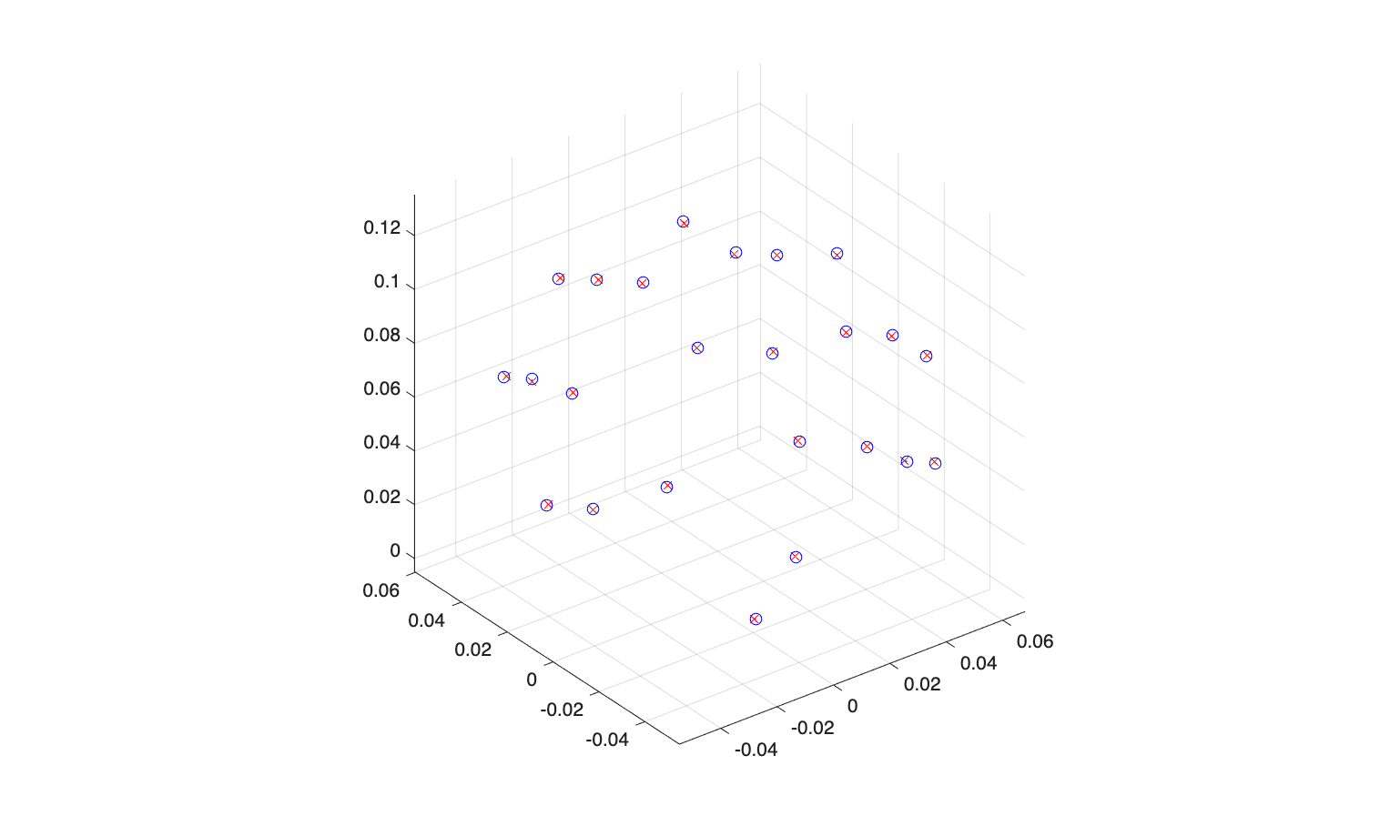
We can plot the positions together and compute the deviations.

figure
ft_plot_sens(fitted,        'elec', false, 'axes', true, 'label', 'off', 'style', 'rx', 'elecsize', 10)
ft_plot_sens(model_aligned, 'elec', false, 'axes', true, 'label', 'off', 'style', 'bo', 'elecsize', 10)

deviation = sqrt(sum((fitted.elecpos - model_aligned.elecpos).^2, 2));
deviation = deviation * 1000; % in mm

figure
bar(deviation);
ylabel('coil number')
ylabel('deviation (mm)')

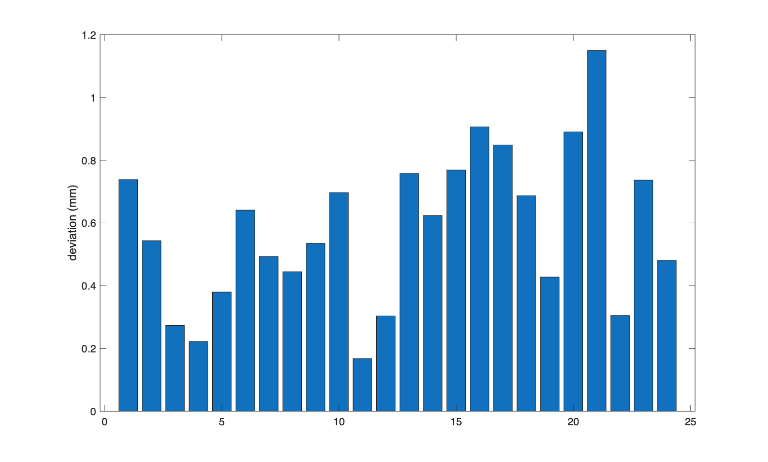
We can see that all but one fitted dipole position is less than 1 mm off from the position that was expected from the CAD model. For a well-functioning SQUID MEG system, localization errors are typically in the range of 1-5 mm (Leahy et al., 1998). For OPM systems, errors of 2-6 mm have been reported depending on the sensor configuration and calibration method (Iivanainen et al., 2022).

Channel gain calibration

Sensor calibration determines the position, orientation, and sensitivity (gain) of each MEG sensor. For SQUID systems this is typically done once during the manufacturing and installation. For OPM systems, where sensors are placed individually and may change position between sessions, calibration needs to be repeated more frequently. The spherical phantom with 24 known coil positions provides a calibration reference: by recording the fields of the coils with the MEG system and fitting a forward model (the magnetic field of a dipole in free space or in a spherical conductor), the sensor parameters can be estimated.

For a single MEG sensor measuring the magnetic field of a single coil, the measured signal depends on:

• The position and orientation of the coil (known from the phantom specification)
• The position and orientation of the sensor (to be determined)
• The gain of the sensor (to be determined)
• The current through the coil (known from the driver settings)

With 24 coils at known positions and the coil currents known, the sensor parameters (position, orientation, gain) can be estimated by minimizing the difference between the measured and predicted field amplitudes across all coils. This is an overdetermined problem (24 measurements for 6 unknowns per sensor), which can be solved by least-squares optimization.

Get the measured and expected fields

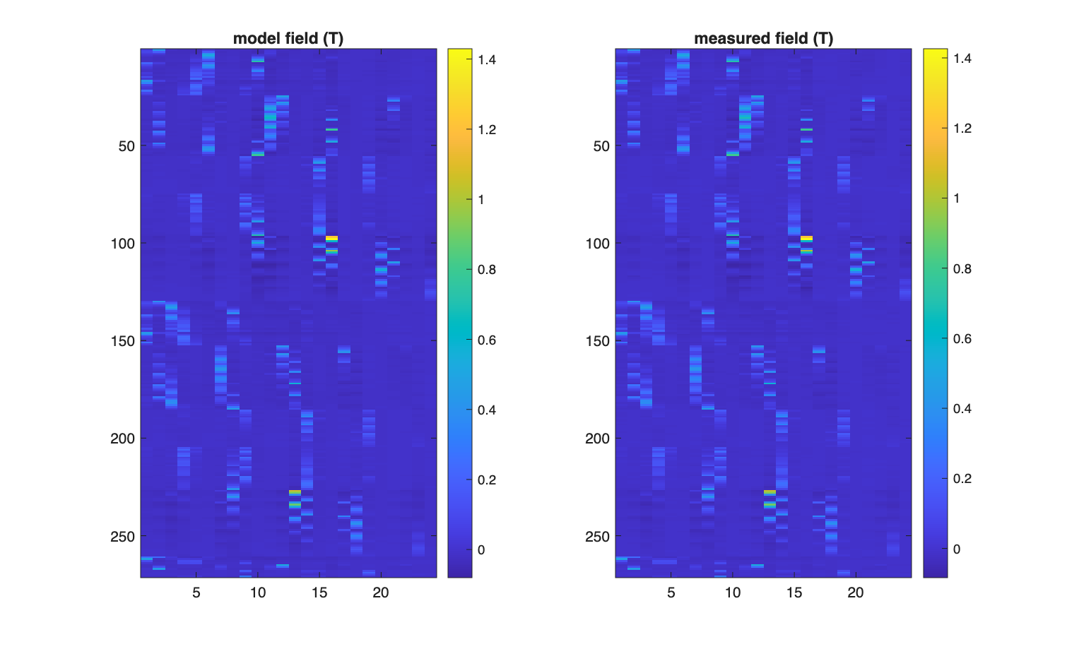
The 24 PCA topographies provide an estimate of how strong each phantom coil is visible on each channel. We can gather them in a Ncoils-by-Nchannels matrix.

clear measured_field
for i=1:24
    measured_field(:,i) = pca{i}.topo * flip(i);
end

We have fitted the topographies of each coil with a magnetic dipole and determined the dipole positions and dipole moment (in Am, or Ampere*meter).

for i=1:24
    coil_pos(i,:) = dip{i}.dip.pos;
    coil_mom(i,:) = dip{i}.dip.mom * flip(i);
end

We can compute the leadfield matrix with the fitted magnetic dipole positions and orientations. The leadfield matrix has three columns for a unit-strength dipole in the x, y, and z-direction. When we multiply the leadfield matrix with the dipole moment, we get the actual field of that coil for each sensor.

% take a subset of MEG channels
cfg = [];
cfg.channel = {'M*'};
grad = ft_electrodeselection(cfg, data.grad);
grad = ft_convert_units(grad, 'm');

clear model_field
for i=1:24
    lf = ft_compute_leadfield(coil_pos(i,:), grad, real_headmodel);
    model_field(:,i) = lf * (coil_mom(i,:)');
end

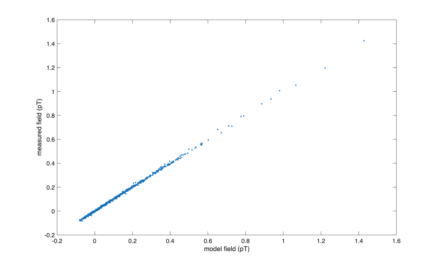
We can plot them as a matrix, or as a scatter plot.

scale = 1e12; % convert from T to pT

figure
subplot(1,2,1); imagesc(model_field*scale);
title('model field (pT)')
colorbar
subplot(1,2,2); imagesc(measured_field*scale);
title('measured field (pT)')
colorbar

figure
plot(model_field(:)*scale, measured_field(:)*scale, '.')
xlabel('model field (pT)')
ylabel('measured field (pT)')

Compute the channel gain

Ideally the measured and the model field would be equal. We can fit a linear model y = b0 + b1*x with an intercept b0 and a slope b1. In this case we know that the intercept must be zero, hence we cannot use the standard MATLAB function polyfit, but instead can use the more general fitlm function from the statistics toolbox.

b1 = zeros(1, 271);
lm = cell(1, 271);
for i=1:271
    x = model_field(i,:);
    y = measured_field(i,:);
    % fit a linear model, using https://nl.mathworks.com/help/stats/wilkinson-notation.html
    lm{i} = fitlm(x,y,'y~x1-1');
    b1(i) = lm{i}.Coefficients.Estimate;
end

b1 = zeros(1, 271);
lm = cell(1, 271);
for i=1:271
    x = model_field(i,:);
    y = measured_field(i,:);
    b1(i) = y/x; % this solves y = b1*x for b1
end

Subsequently we can visualize the gain for each channel.

figure
bar(b1)
xlabel('channel')
ylabel('actual gain')
ylim([0.8 1.2])
grid on

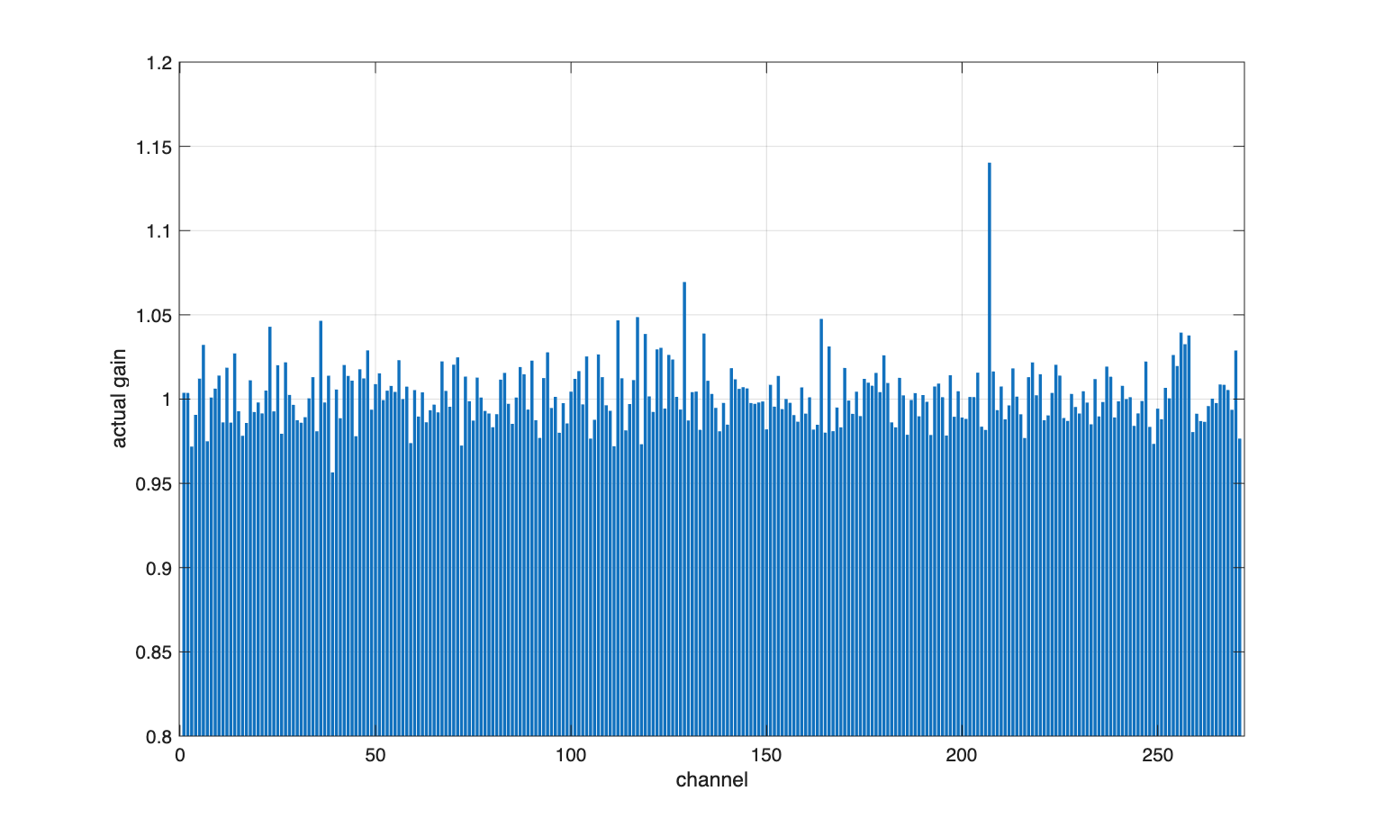
We had expected all of these to be close to one. The mean is one, which is by construct as we don’t know the actual current and precise coil diameter of the 24 dipole coils. The standard deviation is about 0.02 or 2%. There are a few channels that have a deviation of about 5%, and channel 207 (MRP21) has a gain that is 1.14, or 14% larger than expected. We can inspect that channel in more detail.

chansel = 207;
x = model_field(chansel,:);
y = measured_field(chansel,:);

figure
hold on
axis square
grid on

plot(x, y, 'o')
plot(x, x, 'g-')
plot(x, b1(chansel)*x, 'r-')

title(sprintf('channel %d', i))
legend({'measured', 'ideal', 'fitted'}, 'location', 'northwest')

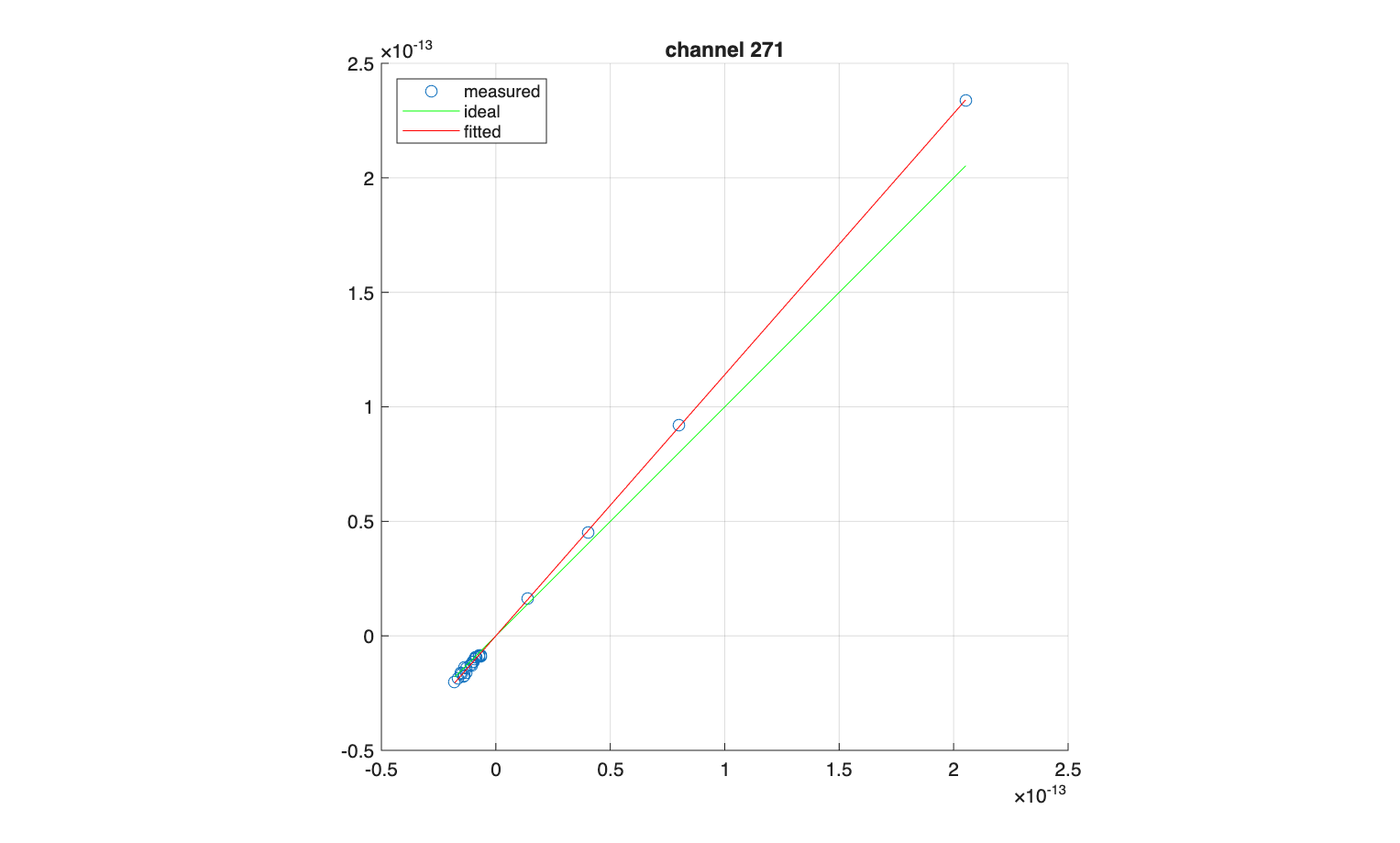
In the upper right corner there is one coil for which this channel has a large value. But if you zoom in on the lower left corner, you can see that it is not just that coil that causes the gain for this channel to be 14% off, the data points for the other coils also fall on the red line and result in a measured value that is 14% larger than expected.

Correcting the channel gain

Now that we know that the channel gain is not as ideal as we would like it to be, we can correct for this. Ideally this is done by the manufacturer, who can modify the channel gain settings in the hardware or acquisition software. But if that is not possible, we can also do it ourselves using a so-called montage. See the ft_prepare_montage and ft_apply_montage functions, or rearch here on the website for the use of a montage. FieldTrip uses the montage for multiple purposes, but basically it is used to do a matrix multiplication of the montage.tra matrix with the data matrix, keeping track of the channel names and ordering (which may be different).

We construct a montage that has one-divided-by-the-gain on the diagonal. This will result in channel 207 being multiplied with 1/1.14.

correctgain = [];
correctgain.tra = diag(1./b1);
correctgain.labelold = grad.label;
correctgain.labelnew = grad.label;

We could now use ft_apply_montage to use this montage on our existing data structure. Alternatively, we can use the montage all the way at the start of the preprocessing pipeline in the ft_preprocessing function.

%% read the raw data and apply the montage to correct the gain
cfg = [];
cfg.dataset = 'phantom_3031000.01_20260721_01.ds';
cfg.continuous = 'yes';
cfg.channel = 'M*'; % only MEG channels
cfg.coilaccuracy = 2; % use the most accurate model for the MEG gradiometers
cfg.montage = correctgain;
data_all = ft_preprocessing(cfg);

Alternatively, we could also use the ft_denoise_synthetic or the ft_denoise_ssp functions, since the CTF synthetic higher-order gradient implementation is also implemented as a montage, as is the signal-space projection method. Both methods require the montage to be part of the grad structure

data.grad.balance.correctgain = correctgain;

% apply the montage using ft_denoise_synthetic
cfg = [];
cfg.gradient = 'correctgain';
cfg.updatesens = 'no';
data_corrected = ft_denoise_synthetic(cfg, data_all);

% apply the montage using ft_denoise_ssp
cfg = [];
cfg.ssp = 'correctgain';
cfg.updatesens = 'no';
data_corrected = ft_denoise_ssp(cfg, data_all);

In principle any linear projection of the data can be considered mathematically similarly, so ft_componentanalysis and ft_rejectcomponent internally also construct and work with montages.

OPM sensor localization

Unlike SQUID systems where the sensor positions are fixed in the dewar, OPM sensors are placed individually in a helmet or a cap and their positions depend on the helmet or cap design, the head size, and the specific sensor placement. Determining the sensor geometry is essential for accurate source reconstruction and for comparing measurements across sessions or participants.

The phantom-based approach has the advantage of directly determining the position and orientation of the sensor’s sensitive point, which is the point where the magnetic field is actually measured. This is more accurate than methods that determine the position of the sensor housing in a CAD model or using a Polhemus digitizer, because the sensitive point (typically the center of the vapor cell and laser) may not coincide with the geometric center of the sensor. Furthermore, the phantom allows to accurately determine the orientation of the vapor cell and laser.

Summary and suggested further reading

This tutorial demonstrated three use cases for a spherical MEG phantom with 24 magnetic dipole coils:

1. System validation: Fitting dipoles to phantom coil signals and comparing the estimated positions with the known ground truth to quantify localization accuracy. This can be used to compare SQUID and OPM systems and to perform routine quality assurance.
2. Channel gain calibration: Using the known coil positions to determine gain of each MEG sensor through least-squares optimization of the measured field amplitudes.
3. OPM sensor localization: Using the phantom to determine the geometry of an OPM sensor array, which is essential for accurate source reconstruction and for comparing coregistration methods.

The 24-coil spherical phantom provides good angular coverage and allows each coil to be driven at a unique frequency, enabling simultaneous measurement of all coils. The Arduino Uno-based current driver provides a flexible and reproducible way to drive the coils.

You may want to continue with the coregistration of OPM data tutorial for more details on aligning OPM sensors with the head, or with the sensitivity maps tutorial to understand how sensor geometry affects MEG sensitivity.

References

• Leahy, R. M., Mosher, J. C., Spencer, M. E., Huang, M. X., & Lewine, J. D. (1998). A study of dipole localization accuracy for MEG and EEG using a human skull phantom. Electroencephalography and Clinical Neurophysiology, 107(2), 159-173. https://doi.org/10.1016/s0013-4694(98)00057-1
• Oyama, D., Adachi, Y., Yumoto, M., Hashimoto, I., & Uehara, G. (2015). Dry phantom for magnetoencephalography — Configuration, calibration, and contribution. Journal of Neuroscience Methods, 251, 24-36. https://doi.org/10.1016/j.jneumeth.2015.05.004
• Cao, F., Gao, Z., Qi, S., Chen, K., Xiang, M., An, N., & Ning, X. (2023). Realistic three-layer head phantom for optically pumped magnetometer-based magnetoencephalography. Computers in Biology and Medicine, 164, 107318. https://doi.org/10.1016/j.compbiomed.2023.107318
• Adachi, Y., Oyama, D., Higuchi, M., & Uehara, G. (2023). A spherical coil array for the calibration of whole-head magnetoencephalograph systems. IEEE Transactions on Instrumentation and Measurement, 72, 1-10. https://doi.org/10.1109/tim.2023.3265750
• Iivanainen, J., Borna, A., Zetter, R., Carter, T. R., Stephen, J. M., McKay, J., et al. (2022). Calibration and localization of optically pumped magnetometers using electromagnetic coils. Sensors, 22(8), 3059. https://doi.org/10.3390/s22083059

See also these tutorials

• Localizing oscillatory sources using beamformer techniques
• Localizing visual gamma and cortico-muscular coherence using DICS
• Analysis of corticomuscular coherence
• Connectivity in auditory evoked responses
• Localizing electrodes using a 3D-scanner
• Creating a BEM volume conduction model of the head for source reconstruction of EEG data
• Creating a FEM volume conduction model of the head for source reconstruction of EEG data
• Creating a volume conduction model of the head for source reconstruction of MEG data
• Introduction to the FieldTrip toolbox
• Source reconstruction of event-related fields using minimum-norm estimation
• Channel and source analysis of mouse EEG
• Comparing MEG sensitivity maps for SQUID and OPM sensor arrays
• Creating a source model for source reconstruction of MEG or EEG data
• Computation of virtual MEG channels in source-space

See also these frequently asked questions

See also these example scripts

• How to select a subset of OPM sensor positions from the 144 slots in the FieldLine smart helmet?
• Designing 3D printed helmets for different OPM sensor types
• Designing an OPM helmet with a straight opening at the bottom