documentation / example / other / opm_selection /

How to select a subset of OPM sensor positions from the 144 slots in the FieldLine smart helmet?

The FieldLine Beta2 smart helmet that we have at the DCCN has 144 slots for OPM sensors. The template gradiometer definition included with FieldTrip lists all those sensor locations, each with a name like L101_bz or R503_bz. The prefix (L or R) indicates the left or right side of the helmet, the three-digit number identifies the sensor location, and the suffix indicates the orientation (_bx, _by, or _bz) of the corresponding channel. With the FieldLine HEDscan v3 system, each OPM sensor can measure the magnetic field in one, two, or three orthogonal directions (bx, by, and bz), so each physical slot corresponds to one, two, or three channels in the data and in the gradiometer definition.

It is recommended to only work with the two orientations by and bz, since the sensitivity of the bx channel is along the direction of the laser and is very noisy.

At the DCCN we currently only have 32 OPM sensors (which means 64 channels) which we can distribute over the 144 slots in the helmet. Depending on your research question you may want to position these 32 sensors uniformly or more clustered over a specific brain region.

The following code demonstrates how to make a graphical selection of the helmet slots in which to place the OPM sensors.

Reading the template sensor positions

You can read the full Beta2 helmet template with all 144 slots using:

grad = ft_read_sens('fieldtrip/template/gradiometer/fieldlinebeta2.mat');

% work in consistent SI units (m, T, V, etc)
grad = ft_convert_units(grad, 'm');

To inspect the helmet layout:

figure
ft_plot_sens(grad, 'fiducial', false)
view([135 20]);

You can rotate the helmet around. Note that the sensors are schematically depicted as circular coils, but in reality each FieldLine OPM sensor is square and 15x13x35 mm in size.

Manual selection of sensor slots

For a specific experiment you will have to decide in which of the 144 slots to place the 32 OPM sensors. A very simple selection would for example be to select every fourth sensor location:

cfg = [];
cfg.channel = 1:4:144; % select every 4th sensor
selected = ft_electrodeselection(cfg, grad); % it also works on MEG sensor descriptions 

figure
ft_plot_sens(selected, 'fiducial', false)

or to select all locations on the left:

cfg = [];
cfg.channel = 'L*'; % starting with L
selected = ft_electrodeselection(cfg, grad);

figure
ft_plot_sens(selected, 'fiducial', false)

We recommend placing at least 5 OPM sensors evenly spaced around the head to keep the helmet in place: one on the vertex, two at the temples, and two at the front and back.

Graphical selection of sensor slots

As demonstrated in the OPM helmet design tutorial, the ft_sensorplacement function can distribute sensors on a 3D printed helmet design. In addition, it returns a 3D model of all sensor positions. This allows us to visualize the sensors with their full spatial extent, and using ft_electrodeselection we can subsequently make a selection.

We trick ft_sensorplacement into using our predefined OPM sensor locations from the template helmet as electrode positions. On each electrode position, it will place an OPM sensor (and the 3D model).

% Construct an electrode-like structure from the OPM gradiometer definition
elec = keepfields(grad, {'unit', 'coordsys'});
elec.type = 'eeg';
elec.label = grad.label;
elec.elecpos = grad.coilpos;  % position of each "electrode" or OPM
elec.elecori = grad.coilori;  % orientation of each "electrode" or OPM

We also need a head surface onto which the electrodes will be projected. We can simply use the electrode (or template OPM) positions instead of a real head surface.

headshape = elec.elecpos;

Finally we need the 3D model of the sensor geometry, which will be copied and placed on each electrode position. You can get the STL file from our download server.

template = ft_read_headshape('fieldline_sensor.stl');
template.unit = 'mm';
template = ft_convert_units(template, 'm');

With these inputs, we can now generate a 3D geometrical description of all sensors. The positions will be the same as the original ones in the template grad structure, but this step will also copy the template STL sensor description to each of the sensor locations for plotting.

cfg = [];
cfg.template = template;
cfg.elec = elec;
[cfg, sensor] = ft_sensorplacement(cfg, headshape);

figure
ft_plot_sens(grad, 'fiducial', false)
ft_plot_mesh(sensor)

Now that we have the 3D model of the 144 sensors, we can plot them in ft_electrodeselection. If the cfg.mesh argument to this function is a struct array with as many elements as the number of sensors in the elec or grad structure, it will plot the 3D models alongside the schematic depiction of the sensors. You can use the MATLAB rotate button to look at the helmet from different angles, and when 3D rotation is off, you can click on an electrode (at the base of each OPM sensor) to enable or disable each sensor.

cfg = [];
cfg.headshape = elec.elecpos;
cfg.mesh = sensor;
selected = ft_electrodeselection(cfg, grad); % click on the sensors to enable/disable them

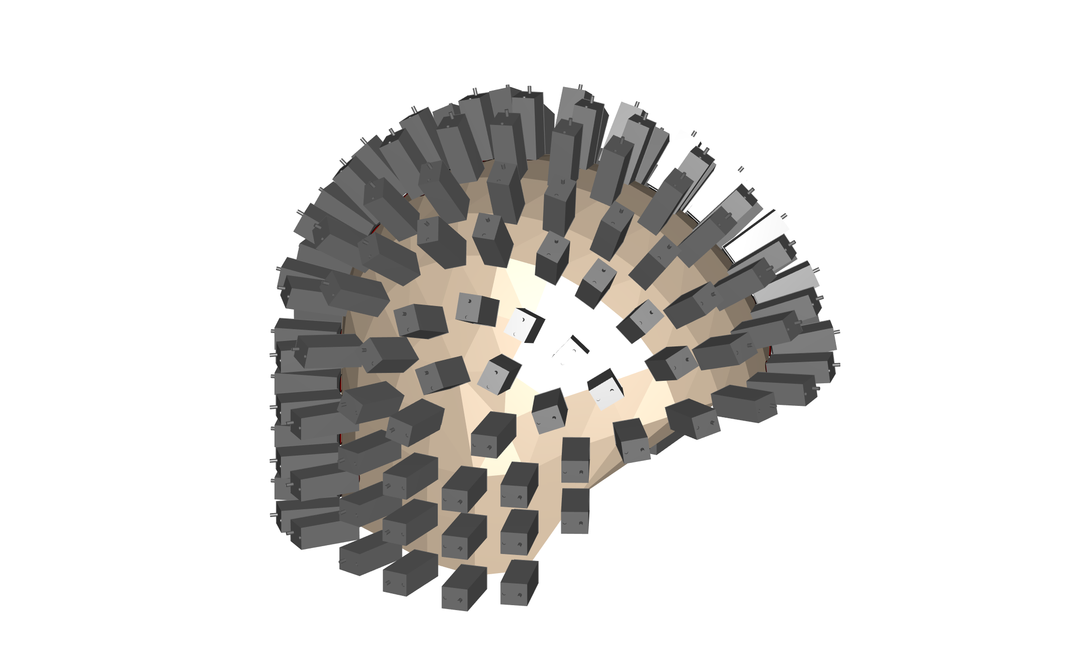
Since we have 144 slots and 32 sensors, we would have to disable 112 of the possible slots. Rather than starting with all sensors enabled, you can also start with only a single sensor enabled. You can subsequently disable that single position by clicking on it, and start selecting the 32 sensor positions from a blank slate. It is not possible to start without any sensor selected, so you should always at least have one channel selected in cfg.channel.

cfg = [];
cfg.headshape = elec.elecpos;
cfg.mesh = sensor;
cfg.channel = 1; % only select the 1st sensor to start with
selected = ft_electrodeselection(cfg, grad); % click on the sensors to enable/disable them

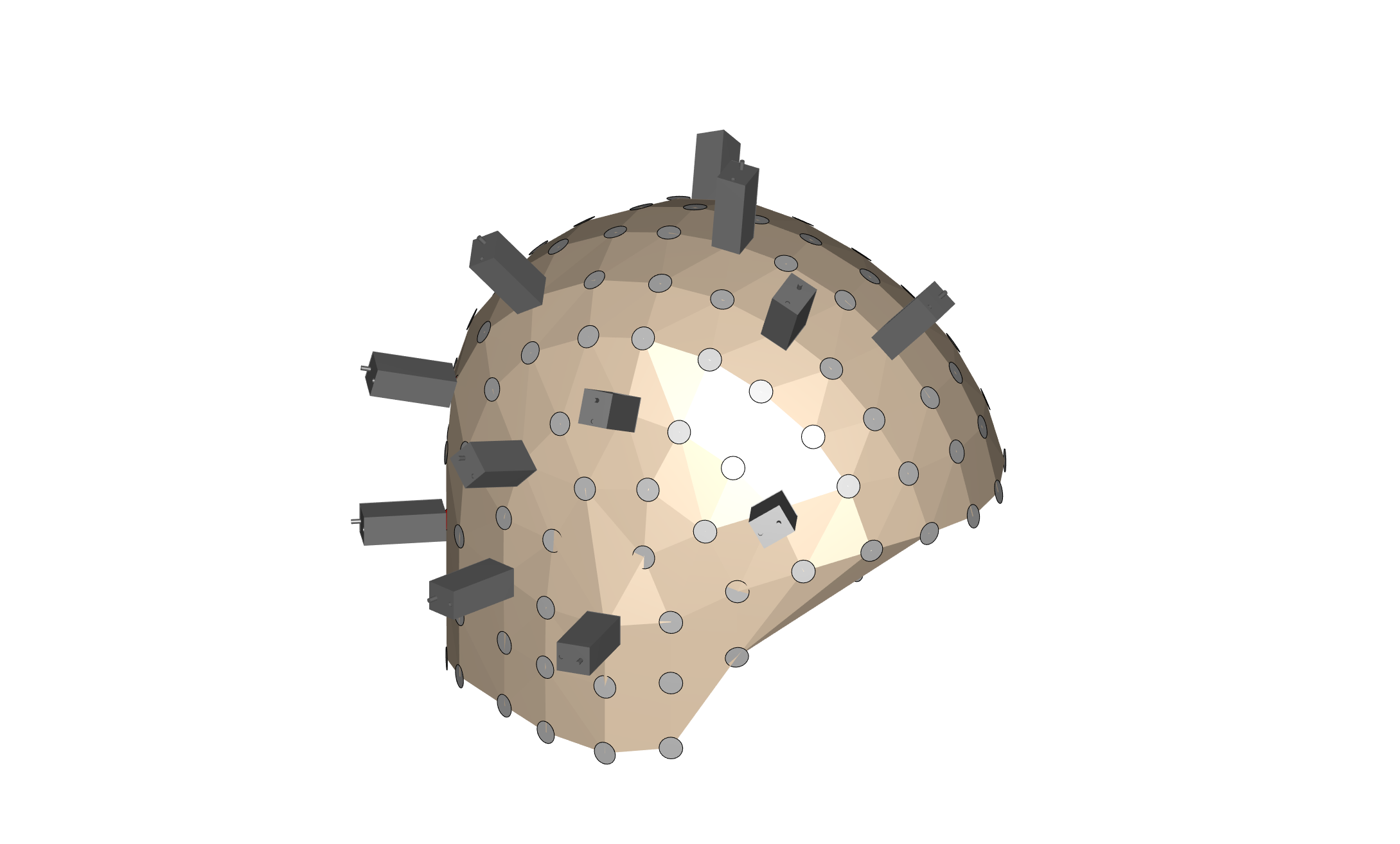
To continue or start from a previously made selection, you can pass its list of channel labels.

cfg = [];
cfg.headshape = elec.elecpos;
cfg.mesh = sensor;
cfg.channel = selected.label; % from the previous iteration
update_selected = ft_electrodeselection(cfg, grad); % click on the sensors to enable/disable them

Making a print-out on paper

For placing the actual sensors it is convenient to bring a paper print-out of the selected channels into the MEG lab. We can use the layout for that:

cfg = [];
cfg.layout = 'fieldtrip/template/layout/fieldlinebeta2bz_helmet.mat';
cfg.skipscale = 'yes';
cfg.skipcomnt = 'yes';
layout_all = ft_prepare_layout(cfg);

cfg = [];
cfg.layout = 'fieldtrip/template/layout/fieldlinebeta2bz_helmet.mat';
cfg.channel = selected.label;
cfg.skipscale = 'yes';
cfg.skipcomnt = 'yes';
layout_selected = ft_prepare_layout(cfg);

for i=1:numel(layout_selected .label)
layout_selected.label{i} = layout_selected.label{i}(1:end-4); % remove the "_bz"
end

This plots all sensor slots as boxes, and the label only for the selected ones.

figure
ft_plot_layout(layout_all, 'box', 'yes', 'label', 'no', 'point', 'no')
hold on
ft_plot_layout(layout_selected, 'box', 'no', 'label', 'yes', 'point', 'no')

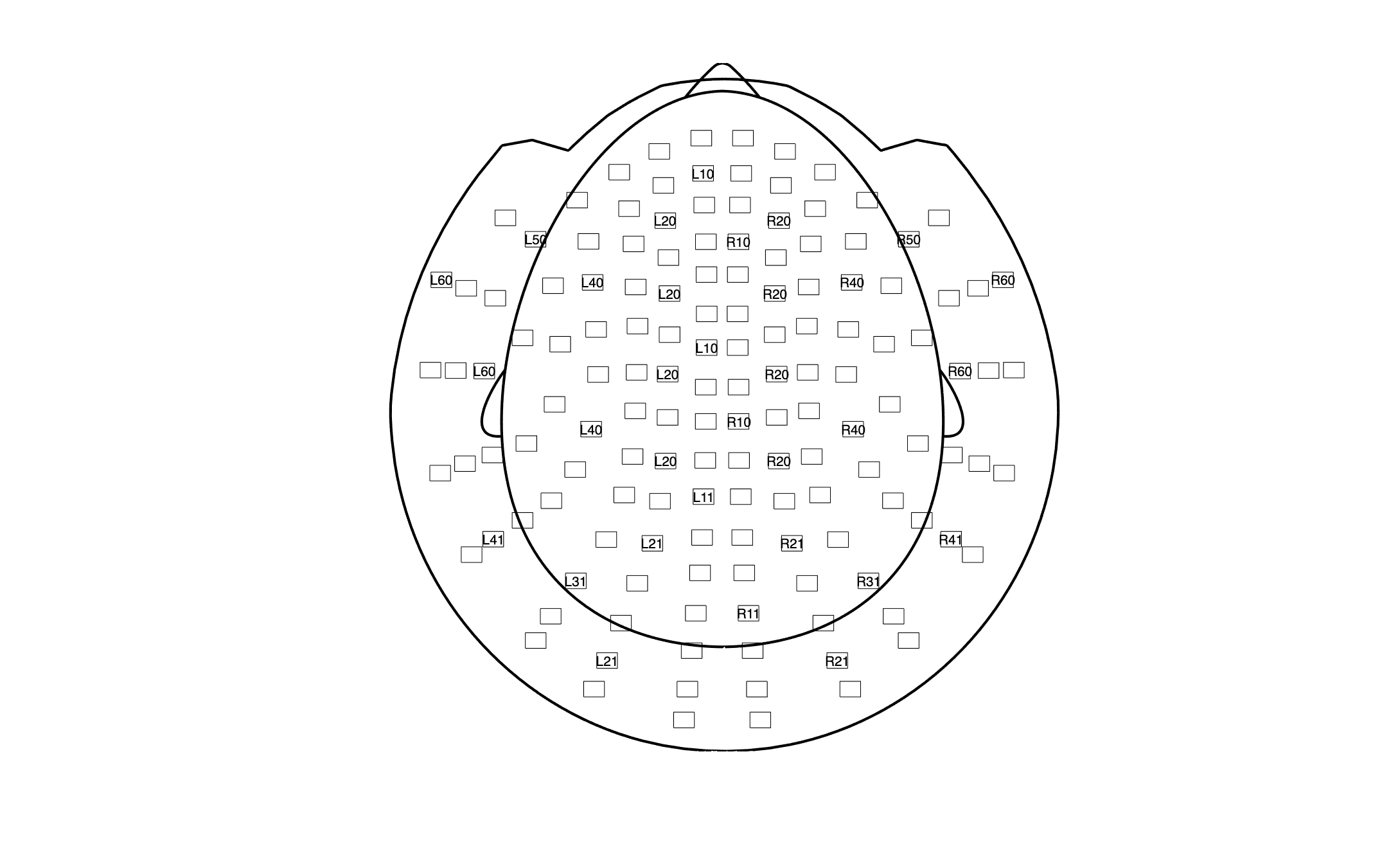
If you will be standing in front of the helmet and participant, you can rotate the labels and turn the page 180 degrees around.

figure
ft_plot_layout(layout_all, 'box', 'yes', 'label', 'no', 'point', 'no')
hold on
ft_plot_layout(layout_selected, 'box', 'no', 'label', 'yes', 'point', 'no', 'labelrotate', 180)

How to select a subset of OPM sensor positions from the 144 slots in the FieldLine smart helmet?

Reading the template sensor positions

Manual selection of sensor slots

Graphical selection of sensor slots

Making a print-out on paper

See also