documentation / tutorial / source / sensitivity_maps /

Comparing MEG sensitivity maps for SQUID and OPM sensor arrays

Introduction

In this tutorial you will learn how to compute and compare the sensitivity of different MEG sensor arrays (both conventional SQUID-based and OPM-based) using the leadfield matrix. The sensitivity for different MEG sensor configurations to dipolar sources on the cortical sheet with either free or fixed dipole orientation is estimated in various ways, allowing for direct comparisons between sensor configurations.

This tutorial assumes that you are familiar with the basic concepts of MEG source reconstruction, including leadfield computation and volume conduction models. You should also be comfortable with the core FieldTrip data structures and functions as covered in the getting started tutorials.

This tutorial does not cover how to use the sensitivity maps for actual source reconstruction of experimental data, nor does it go into detail into the different levels of sensor noise or sensitivity to environmental noise. For source reconstruction methods, see the beamforming and minimum-norm estimate tutorials.

Background

The strength of the measured MEG signal is determined by the magnitude of the leadfield at a certain channel for a given dipole position and orientation. The leadfield matrix represents these magnitudes for all channels (and optionally for all three orientations), and it can be plotted topographically over the MEG helmet. By computing the singular value decomposition (SVD) of the leadfield matrix at each source location, we can quantify the sensitivity as a function of position across the cortex.

We know that in the orientation of the dentritic tree of the neurons that we pick up with EEG and MEG is perpendicular to the cortical sheet. This can be used as constraint for source reconstruction, althogh often in practice this is not done as it requires an accurate individual cortical sheet and good coregistration of the MEG sensors with the head. However, in these simulations we can use the cortical orientation constraint. For each source position, we can compute two measures:

Free-orientation sensitivity: the largest singular value of the full 3-column leadfield matrix, representing the maximum sensitivity achievable with optimal dipole orientation.
Fixed-orientation sensitivity: the norm of the leadfield projected onto the known cortical surface normal, representing the sensitivity for sources oriented perpendicular to the cortical surface.

Additionally, we compute the distance from each dipole on the cortical sheet to the nearest sensor, which helps explain the spatial pattern of sensitivity.

Procedure

To compute and compare the sensitivity maps for different MEG sensor arrays, we will perform the following steps:

Load a segmented MRI, create a scalp surface and a volume conduction model using ft_prepare_headmodel
Load a cortical sheet source model using ft_read_headshape
Load and align the CTF sensor arrays (64, 151, 275 channels) using ft_read_sens and ft_electroderealign
Compute the leadfield matrices using ft_prepare_leadfield
Compute the sensitivity maps using ft_sensitivitymap
Visualize the sensitivity maps for individual arrays and compare across arrays
Repeat the analysis for the FieldLine beta2 OPM array

Prepare the head model and sensors

The anatomical data that we will be working with is based on the canonical MRI of SPM, also known as the “colin27” brain. This is a high-quality, average MRI scan of a single person’s brain that was created by combining 27 scans of the same individual, aligned to the MNI152 atlas. The anatomical data is included with FieldTrip in the template directory.

Load the volume conduction model and source model

We start by reading an MRI segmentation (which already contains scalp, skull, and brain compartments) and a cortical sheet source model. All are in MNI/SPM coordinates.

% these are all in MNI/SPM coordinates
mri_segmented = ft_read_mri('standard_seg.mat');
mri_segmented.coordsys = 'mni';

sourcemodel = ft_read_headshape('cortex_20484.surf.gii'); % there are also lower resolution models

% ensure that all are in mm
mri_segmented = ft_convert_units(mri_segmented, 'mm');
sourcemodel   = ft_convert_units(sourcemodel, 'mm');

Visualize the segmentation

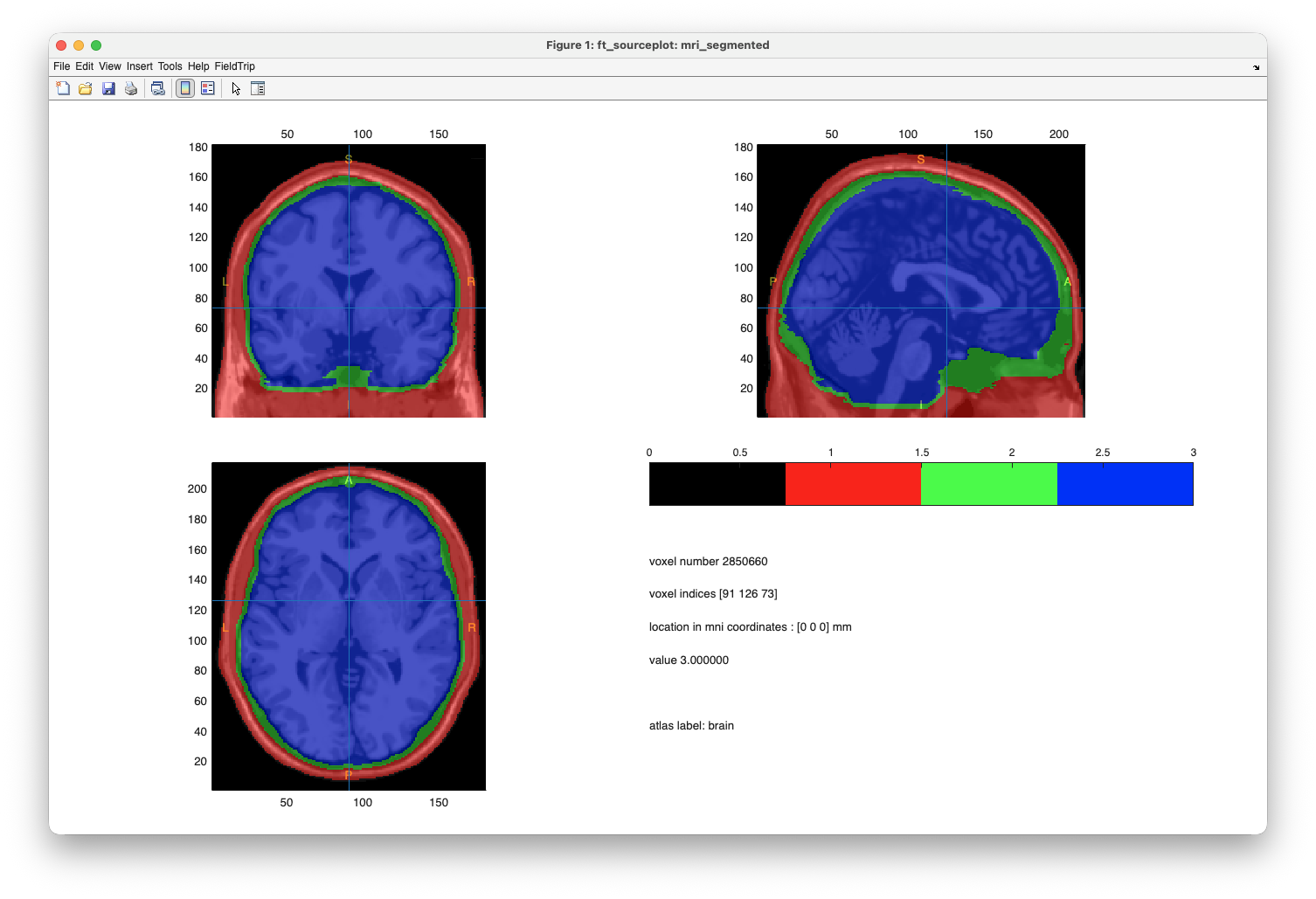
The segmentation contains scalp, skull, and brain compartments. This can be converted to an atlas-like representation to allow clicking and showing the tissue labels.

% combined with cfg.atlas, this allows for clicking and showing the tissue label
mri_segmented.seglabel = {'scalp', 'skull', 'brain'};

cfg = [];
cfg.anaparameter = 'anatomy';
cfg.funparameter = 'seg';
cfg.funcolormap = [
    0 0 0 % black
    1 0 0 % red
    0 1 0 % green
    0 0 1 % blue
    ];
cfg.atlas = mri_segmented;
cfg.location = [0 0 0];
ft_sourceplot(cfg, mri_segmented)

Create the scalp mesh

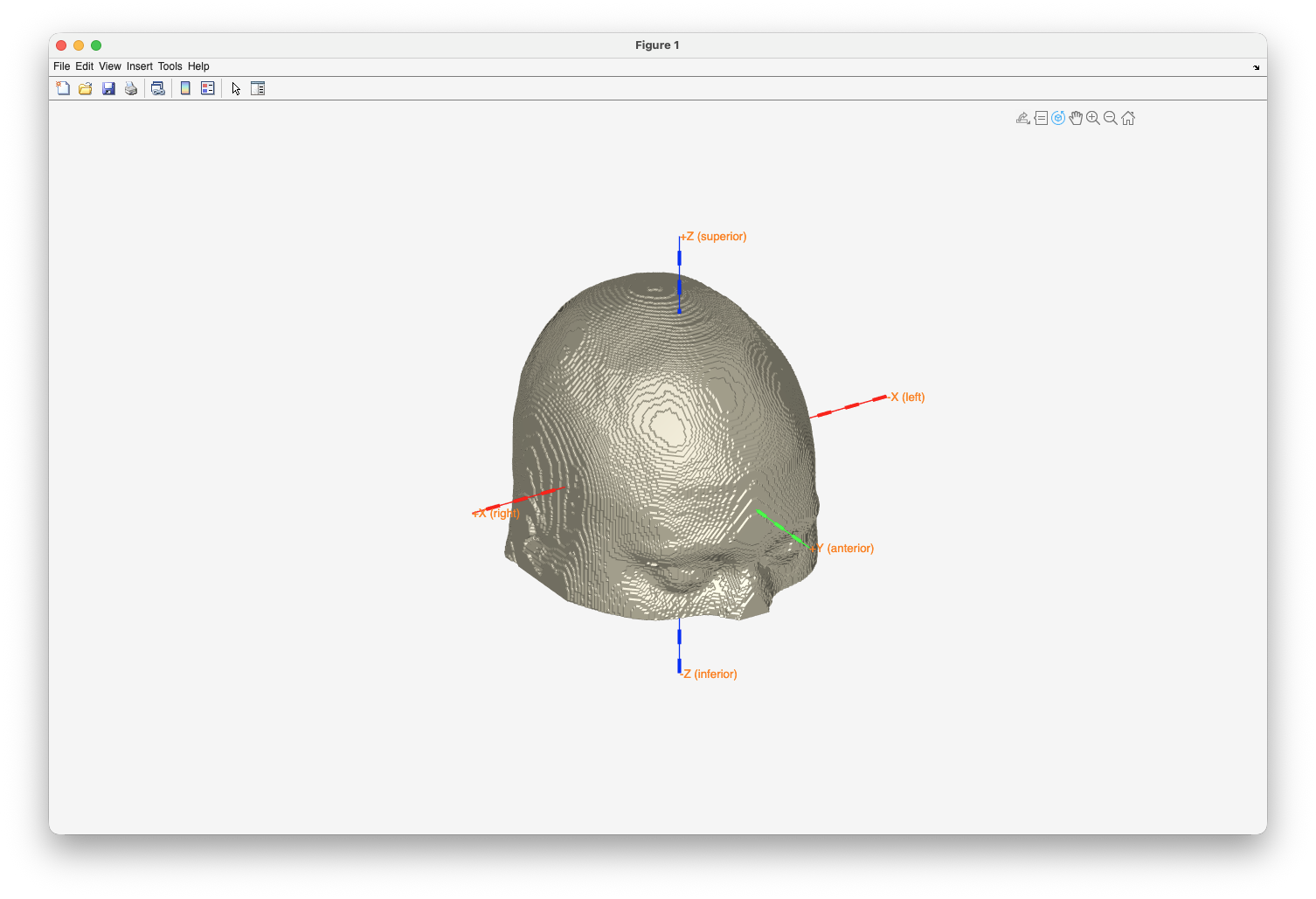
We extract the scalp surface as a high-resolution mesh using an isosurface.

cfg = [];
cfg.tissue = 'scalp';
cfg.method = 'isosurface';
cfg.numvertices = inf;
scalp = ft_prepare_mesh(cfg, mri_segmented);

ft_plot_mesh(scalp, 'axes', true)
ft_headlight

Create the volume conduction model

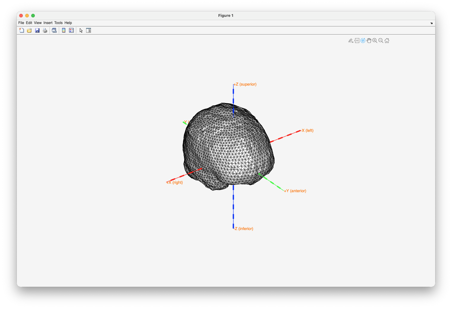
We create a single-shell volume conduction model for MEG from the brain compartment.

cfg = [];
cfg.tissue = 'brain';
cfg.method = 'singleshell';
headmodel = ft_prepare_headmodel(cfg, mri_segmented);

ft_plot_headmodel(headmodel, 'axes', true)
ft_headlight

Load the sensor arrays

We load several CTF SQUID sensor arrays with 275, 151 and 64 channels.

ctf64 = ft_read_sens('ctf64.mat');
ctf64 = ft_convert_units(ctf64, 'mm');

ctf151 = ft_read_sens('ctf151.mat');
ctf151 = ft_convert_units(ctf151, 'mm');

ctf275 = ft_read_sens('ctf275.mat');
ctf275 = ft_convert_units(ctf275, 'mm');

The 64-channel CTF system was the first whole-head system that they built and it dates back to the ’90s, see Vrba et al. (1993) “Whole cortex, 64 channel SQUID biomagnetometer system”. The 151-channel system was the first MEG system to be installed at the Donders and data from that system is also used elsewhere in the FieldTrip tutorials. The 275-channel CTF system was installed at the Donders around 2008.

Select the MEG channels

For the CTF systems we select only the MEG channels, excluding the reference channels.

cfg = [];
cfg.channel = {'S*'}; % regular channels in this system start with an S
ctf64 = ft_electrodeselection(cfg, ctf64); % this also works for gradiometer structures

cfg = [];
cfg.channel = {'M*'};
ctf151 = ft_electrodeselection(cfg, ctf151); % this also works for gradiometer structures

cfg = [];
cfg.channel = {'M*'};
ctf275 = ft_electrodeselection(cfg, ctf275); % this also works for gradiometer structures

Plot the sensors together

figure
ft_plot_sens(ctf64);
ft_plot_sens(ctf151);
ft_plot_sens(ctf275);

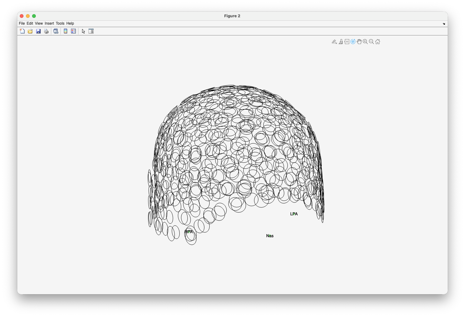
We can see that the three sensor arrays are aligned to each other. Each of the sensor arrays also includes the default/template locations of the Nasion and LPA/RPA anatomical landmarks or fiducials.

Align the sensors to the head model

The different CTF systems are aligned to themselves, but not to the MNI coordinate system of the template headmodel and cortical sheet. The CTF sensors therefore need to be interactively aligned to the head. We can do this for the 275-channel system.

cfg = [];
cfg.method = 'interactive';
cfg.headshape = scalp;
ctf275_aligned = ft_electroderealign(cfg, ctf275);

In the interactive alignment you should rotate and translate the sensor array to match the head surface. You can use the following rotations and translations:

rotate around x +8
rotate around z +90
translate along y -40
translate along z -35
apply
quit

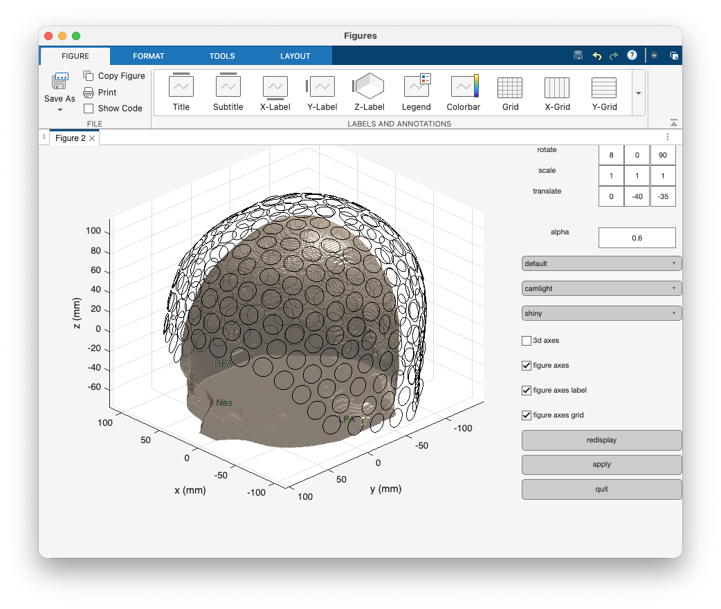
The CTF151 and CTF64 arrays are similarly aligned, so you can use the same transformation for those.

disp(ctf275_aligned.homogeneous)

transform = [
    0.0000   -1.0000    0.0000    0.0000
    0.9903    0.0000   -0.1392  -40.0000
    0.1392    0.0000    0.9903  -35.0000
        0         0         0     1.0000
  ];

The following ensures that all three are similarly aligned to the head in MNI coordinates.

ctf64_aligned  = ft_transform_geometry(transform, ctf64, 'homogeneous');
ctf151_aligned = ft_transform_geometry(transform, ctf151, 'homogeneous');
ctf275_aligned = ft_transform_geometry(transform, ctf275, 'homogeneous');

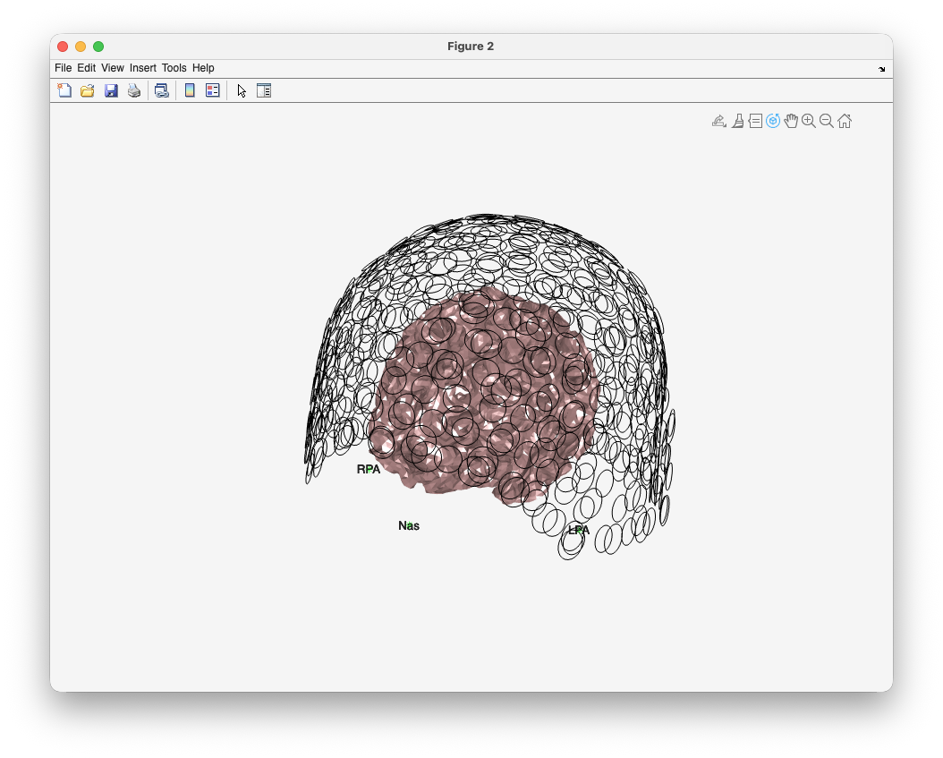
You can check the alignment by plotting the sensors with the cortical surface.

figure
ft_plot_sens(ctf64_aligned);
ft_plot_sens(ctf151_aligned);
ft_plot_sens(ctf275_aligned);
ft_plot_headshape(sourcemodel, 'facecolor', [0.8 0.6 0.6]);
ft_headlight

Convert to SI units

For correct numerical computation of the leadfields, everything should be in SI units (meters, Tesla, etc.).

sourcemodel     = ft_convert_units(sourcemodel, 'm');
headmodel       = ft_convert_units(headmodel, 'm');
scalp           = ft_convert_units(scalp, 'm');
ctf64_aligned   = ft_convert_units(ctf64_aligned, 'm');
ctf151_aligned  = ft_convert_units(ctf151_aligned, 'm');
ctf275_aligned  = ft_convert_units(ctf275_aligned, 'm');

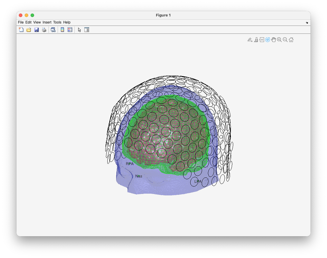
You can plot the sensors, head, and cortical surface together to confirm everything is properly aligned.

ft_plot_mesh(sourcemodel, 'edgecolor', 'none', 'facecolor', 'r')
ft_plot_mesh(headmodel.bnd, 'edgecolor', 'g', 'facealpha', 0.5)
ft_plot_mesh(scalp, 'edgecolor', 'none', 'facecolor', 'b', 'facealpha', 0.2)
ft_plot_sens(ctf275_aligned, 'coil', false, 'orientation', false)
ft_headlight

Compute the leadfield

We compute the leadfield for each of the sensor arrangements. The inside field is set to all ones to indicate that all sources are inside the volume conduction model.

cfg = [];
cfg.headmodel = headmodel; % singleshell model for MEG
cfg.sourcemodel = sourcemodel; % cortical sheet
cfg.sourcemodel.inside = ones(size(sourcemodel.pos,1), 1);
cfg.orientation = 'yes'; % compute the dipole orientations

cfg.grad = ctf64_aligned;
sourcemodel_ctf64 = ft_prepare_leadfield(cfg);

cfg.grad = ctf151_aligned;
sourcemodel_ctf151 = ft_prepare_leadfield(cfg);

cfg.grad = ctf275_aligned;
sourcemodel_ctf275 = ft_prepare_leadfield(cfg);

Compute sensitivity from the leadfield

We compute the sensitivity maps by looping over all source positions and by computing the sensitivity for each dipole using the SVD. For free orientation we take the largest singular value of the full leadfield matrix. For fixed orientation we project the leadfield onto the known cortical surface normal and compute its norm. Since we need to compute the sensitivity maps for multiple senmsor arrays, it is convenient to make that code in a separate function.

Copy the following code and paste it in a local MATLAB file ft_sensitivitymap.m that you save on your own computer.

function sourcemodel = ft_sensitivitymap(cfg, sourcemodel)

% FT_SENSITIVITYMAP computes various measures of sensitivity

sourcemodel.free     = nan(size(sourcemodel.pos,1), 1);
sourcemodel.fixed    = nan(size(sourcemodel.pos,1), 1);
sourcemodel.distance = nan(size(sourcemodel.pos,1), 1);

% ensure that it has chanpos
cfg.grad = ft_datatype_sens(cfg.grad);

for i=1:size(sourcemodel.pos,1)
[u, s, v] = svd(sourcemodel.leadfield{i}, 'econ');
sourcemodel.free(i) = s(1);

[u, s, v] = svd(sourcemodel.leadfield{i} * (sourcemodel.ori(i,:)'), 'econ');
sourcemodel.fixed(i) = s(1);

% compute the distance of all channels to this source
d = cfg.grad.chanpos;
d(:,1) = d(:,1) - sourcemodel.pos(i,1);
d(:,2) = d(:,2) - sourcemodel.pos(i,2);
d(:,3) = d(:,3) - sourcemodel.pos(i,3);
d = sqrt(sum(d.^2, 2));

sourcemodel.distance(i) = min(d); % take the smallest distance
end

% only keep the relevant fields
sourcemodel = keepfields(sourcemodel, {'pos', 'tri', 'ori', 'unit', 'free', 'fixed', 'distance'});

We can now use the local function to compute the sensitivity maps for the different CTF sensor arrays.

cfg = [];
cfg.grad = ctf275_aligned;
sensitivity_ctf275 = ft_sensitivitymap(cfg, sourcemodel_ctf275);

cfg.grad = ctf151_aligned;
sensitivity_ctf151 = ft_sensitivitymap(cfg, sourcemodel_ctf151);

cfg.grad = ctf64_aligned;
sensitivity_ctf64 = ft_sensitivitymap(cfg, sourcemodel_ctf64);

Visualize the sensitivity maps

Distance to the nearest sensor

figure
title('distance (mm)')
ft_plot_mesh(sourcemodel, 'vertexcolor', sensitivity_ctf275.distance * 1e3)
ft_plot_sens(ctf275_aligned)
ft_colormap('RdBu') % from red (low values) to blue (high values)
colorbar
view([-139 11])

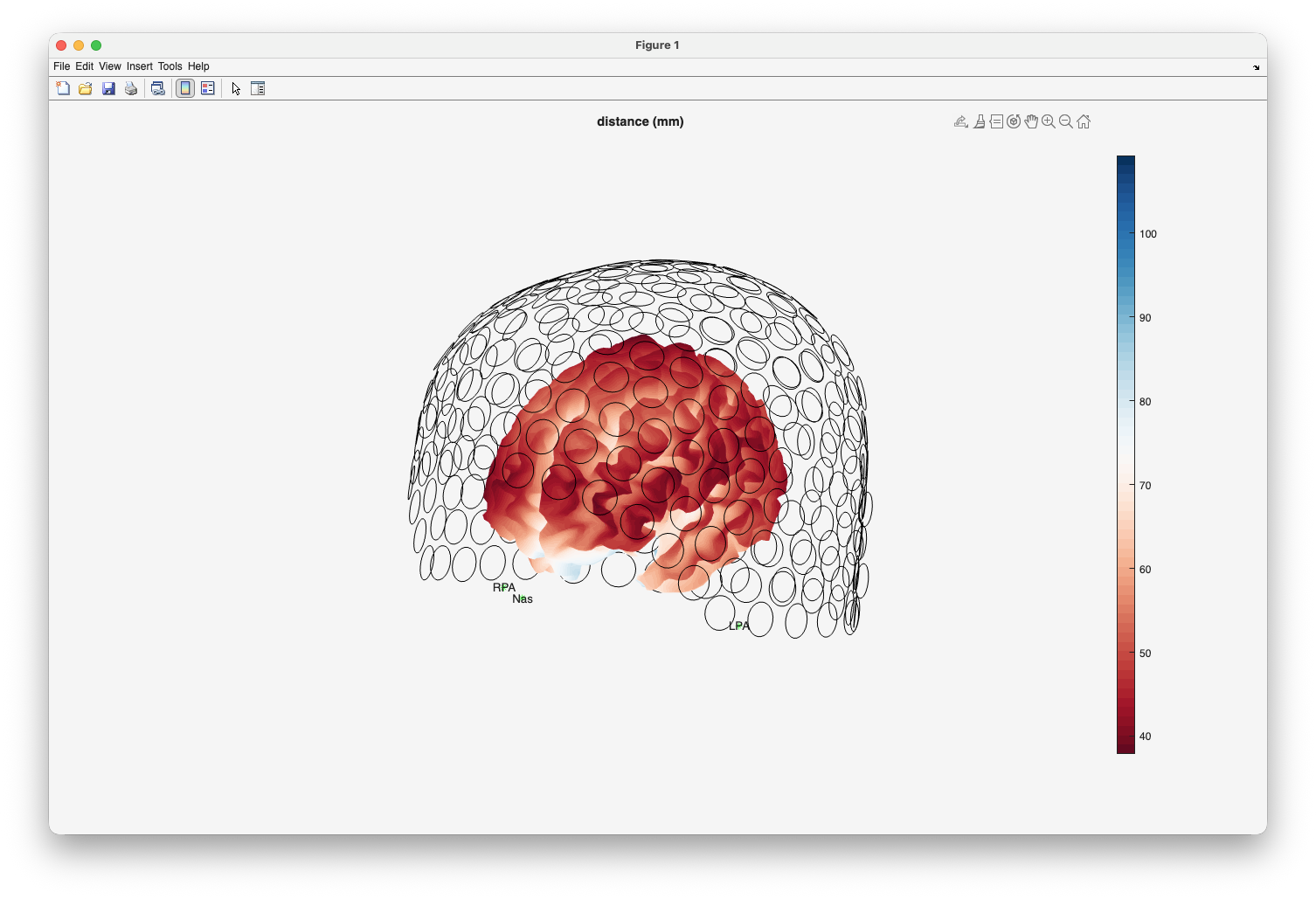
If you rotate it so that you can see the bottom of the brain, you can see that distance to the deep sources is the largest which is here coded in blue.

Relative sensitivity (free orientation)

figure
title('relative sensitivity, orientation free')
ft_plot_mesh(sourcemodel, 'vertexcolor', sensitivity_ctf275.free./max(sensitivity_ctf275.free))
ft_plot_sens(ctf275_aligned)
ft_colormap('-RdBu') % from red to blue, but then the opposite
clim([0 1])
colorbar
view([-139 11])

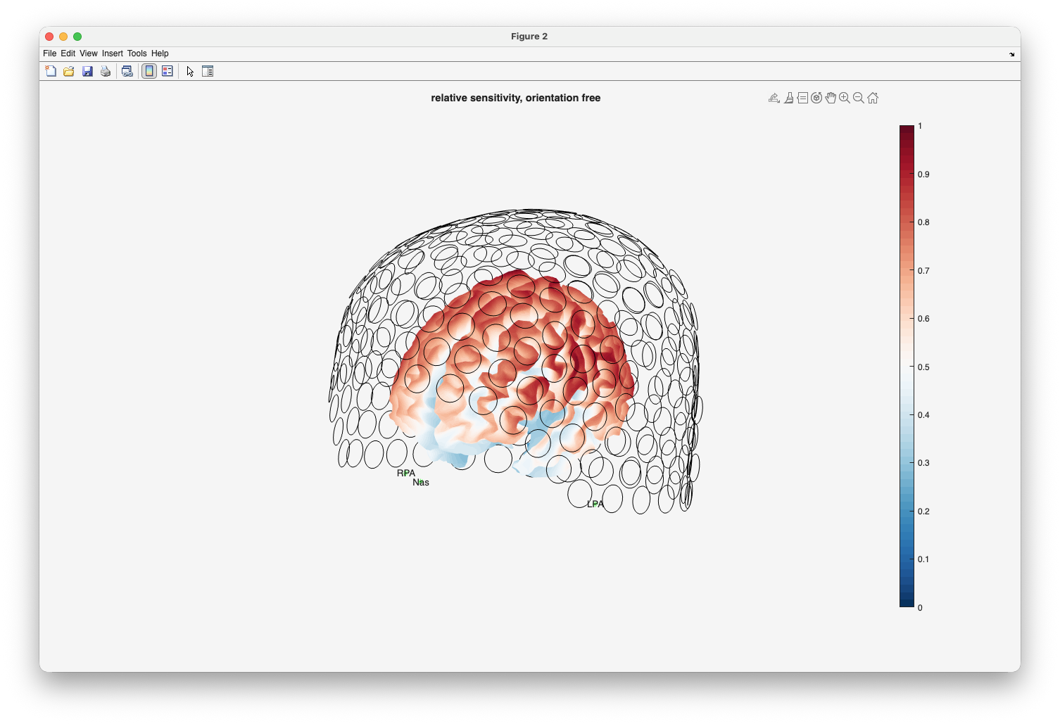
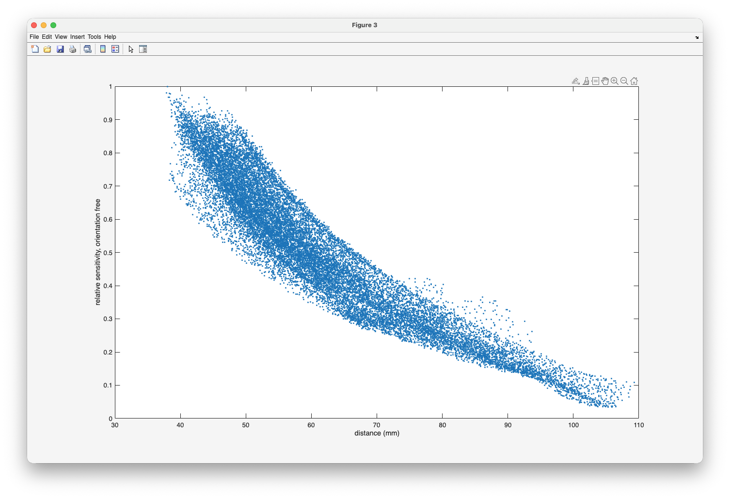
The sensitivity decreases for the deeper sources. We can also plot the sensitivity as a function of distance.

figure
plot(sensitivity_ctf275.distance * 1e3, sensitivity_ctf275.free./max(sensitivity_ctf275.free), '.')
xlabel('distance (mm)');
ylabel('relative sensitivity, orientation free');

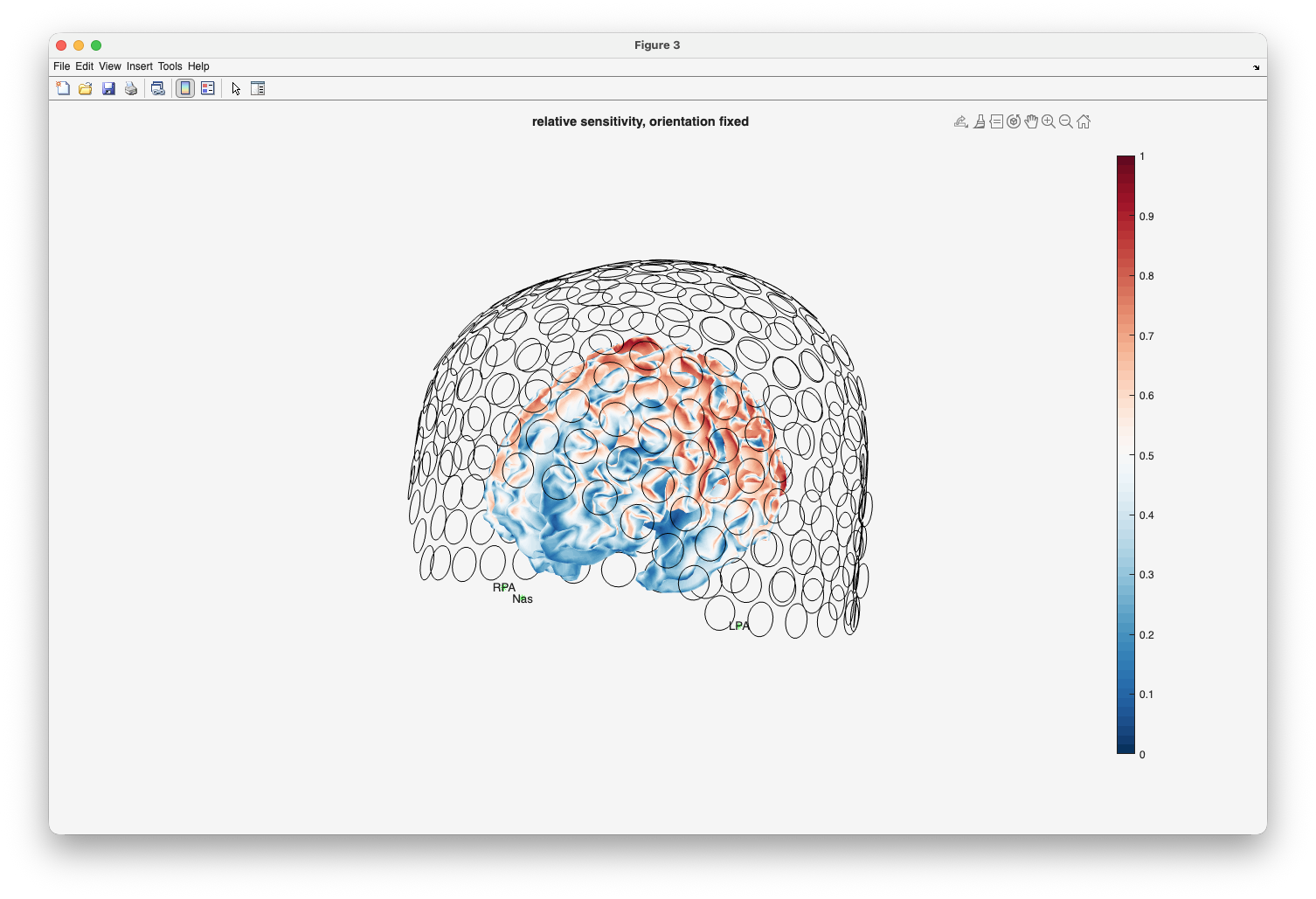
Relative sensitivity (fixed orientation)

figure
title('relative sensitivity, orientation fixed')
ft_plot_mesh(sourcemodel, 'vertexcolor', sensitivity_ctf275.fixed./max(sensitivity_ctf275.fixed))
ft_plot_sens(ctf275_aligned)
ft_colormap('-RdBu') % from red to blue, but then the opposite
clim([0 1])
colorbar
view([-139 11])

Absolute sensitivity (fixed orientation)

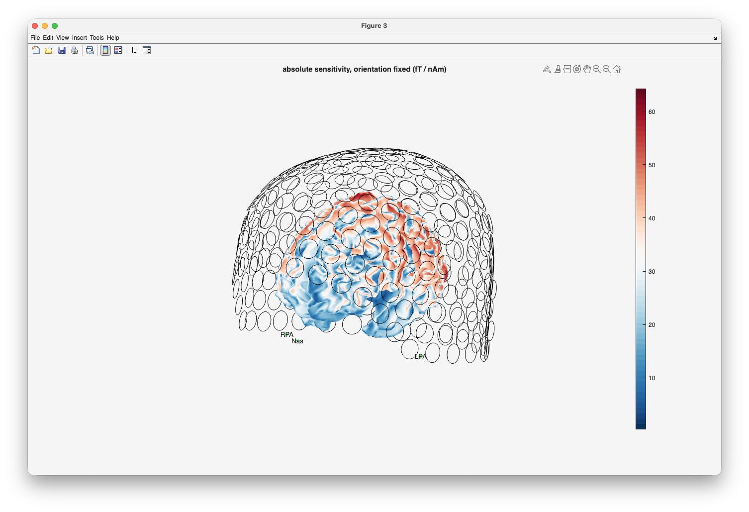
The relative sensitivity is scaled relative to that of the most sensitive dipole, which is useful to compare the sensitivity over the cortical sheet. However, if we want to compare the sensitivity between different sensor arrays, we need to use the absolute sensitivy. The leadfield values are in T/Am. To convert these to the more intuitive fT/nAm, we multiply by 1e15 (T to fT) and divide by 1e-9 (A to nA), which is equivalent to multiplying by 1e6.

figure
title('absolute sensitivity, orientation fixed (fT / nAm)')
ft_plot_mesh(sourcemodel, 'vertexcolor', sensitivity_ctf275.fixed * 1e6)
ft_plot_sens(ctf275_aligned)
ft_colormap('-RdBu') % from red to blue, but then the opposite
colorbar
view([-139 11])

Compare sensitivity between CTF systems

We can now directly compare between the different CTF systems.

figure

h1 = subplot(1,3,1); title('ctf64')
ft_plot_mesh(sourcemodel, 'vertexcolor', sensitivity_ctf64.fixed * 1e6)
ft_plot_sens(ctf64_aligned, 'edgealpha', 0.3)
ft_colormap('-RdBu') % from red to blue, but then the opposite
colorbar
clim([0 60])

h2 = subplot(1,3,2); title('ctf151')
ft_plot_mesh(sourcemodel, 'vertexcolor', sensitivity_ctf151.fixed * 1e6)
ft_plot_sens(ctf151_aligned, 'edgealpha', 0.3)
ft_colormap('-RdBu') % from red to blue, but then the opposite
colorbar
clim([0 60])

h3 = subplot(1,3,3); title('ctf275')
ft_plot_mesh(sourcemodel, 'vertexcolor', sensitivity_ctf275.fixed * 1e6)
ft_plot_sens(ctf275_aligned, 'edgealpha', 0.3)
ft_colormap('-RdBu') % from red to blue, but then the opposite
colorbar
clim([0 60])

linkprop([h1, h2, h3], {"CameraPosition","CameraUpVector"});
view([-139 11])
rotate3d

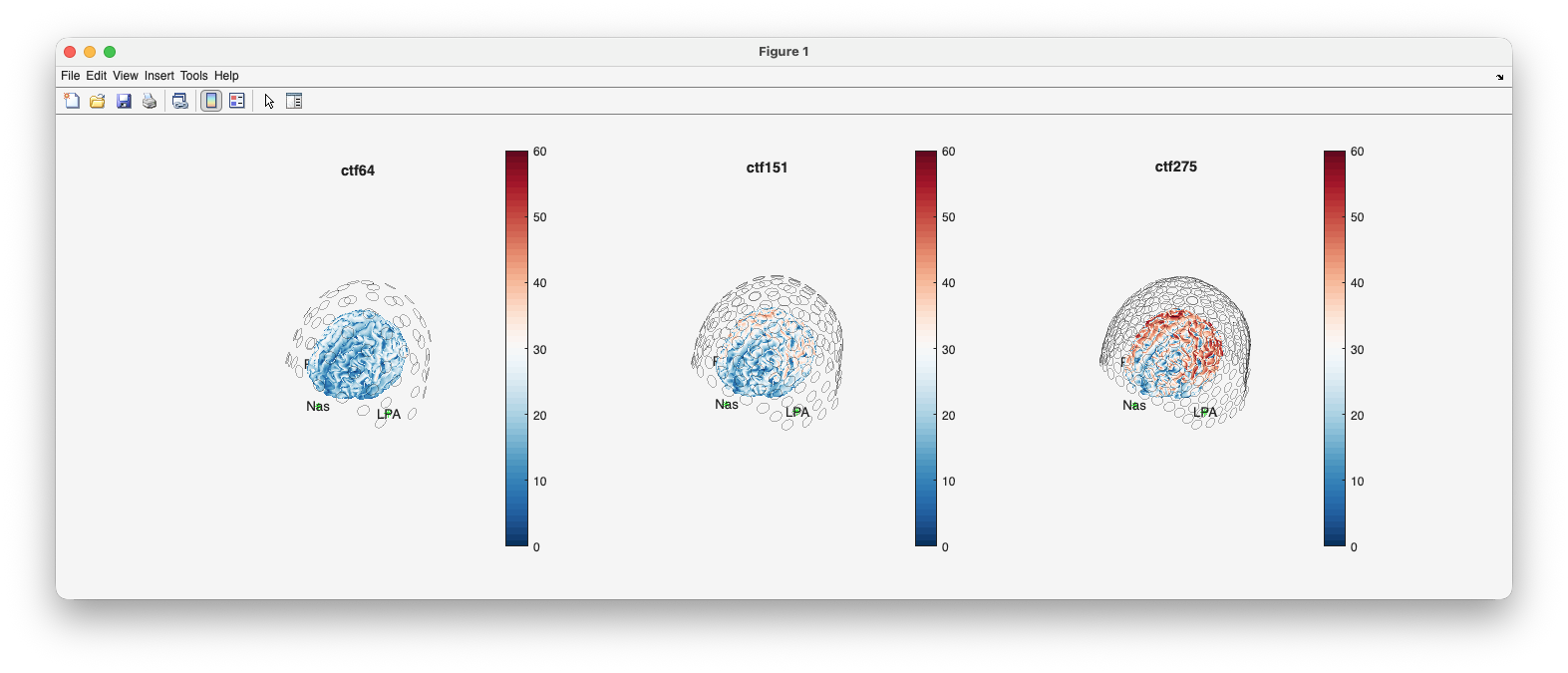
Even though the distance of the sensors to the sources is not really different for the 64, 151 and 275 channel systems, the increase in the number of channels has a considerable impact on the sensitivity.

Compute OPM sensitivity maps

We can also compute the sensitivity map for the FieldLine beta2 OPM sensor array.

fieldlinebeta2 = ft_read_sens('fieldlinebeta2.mat');
fieldlinebeta2 = ft_convert_units(fieldlinebeta2, 'mm');

This again needs to be aligned with the MNI template head.

cfg = [];
cfg.method = 'interactive';
cfg.headshape = scalp;
fieldlinebeta2_aligned = ft_electroderealign(cfg, fieldlinebeta2);

The FieldLine template helmet is already rotated consistently with the MNI head, it only needs a bit of translation which you can achieve with the following steps:

transform along y with -20 mm
transform along z with +10 mm
apply
quit

Then convert to SI units.

fieldlinebeta2_aligned  = ft_convert_units(fieldlinebeta2_aligned, 'm');

OPM sensors are flexible in their placement and the FieldLine smart helmet allows each OPM sensor to slide inwards so that the bottom of the sensor touches the scalp. The FieldLine template sensor positions therefore need to be shifted inwards to match the real distance to the scalp and brain. To determine the amount by which to shift the sensors towards the scalp, we compute the distance of each sensor to the nearest point on the (high-resolution) scalp surface. Subsequently we shift the sensors inward along their orientation vectors.

The FieldLine sensor has a 5 mm standoff distance: the center of the cell (where the laser is) is offset 5 mm from the base of the sensor housing. So the position where the measurement is done (and the leadfield is modelled) should be 5 mm from the scalp surface.

% estimate the distance to the scalp
d = nan(144,1);
for i=1:144
  tmp = scalp.pos;
  tmp(:,1) = tmp(:,1) - fieldlinebeta2_aligned.coilpos(i,1);
  tmp(:,2) = tmp(:,2) - fieldlinebeta2_aligned.coilpos(i,2);
  tmp(:,3) = tmp(:,3) - fieldlinebeta2_aligned.coilpos(i,3);
  tmp = sqrt(sum(tmp.^2,2));

  d(i) = min(tmp); % shortest distance
end

% correct for the 5 mm standoff distance of the FieldLine sensors
d = d - 0.005;

% don't confuse channels and coils, which happen to be the same here
% the chanpos will be automatically recomputed if needed
fieldlinebeta2_shifted = removefields(fieldlinebeta2_aligned ,{'chanpos', 'chanori', 'fid'});

for i=1:144
  fieldlinebeta2_shifted.coilpos(i,:) = fieldlinebeta2_shifted.coilpos(i,:) - d(i) * fieldlinebeta2_shifted.coilori(i,:);
end

figure
ft_plot_sens(fieldlinebeta2_shifted);
ft_plot_headshape(scalp, 'facecolor', 'skin');
ft_headlight

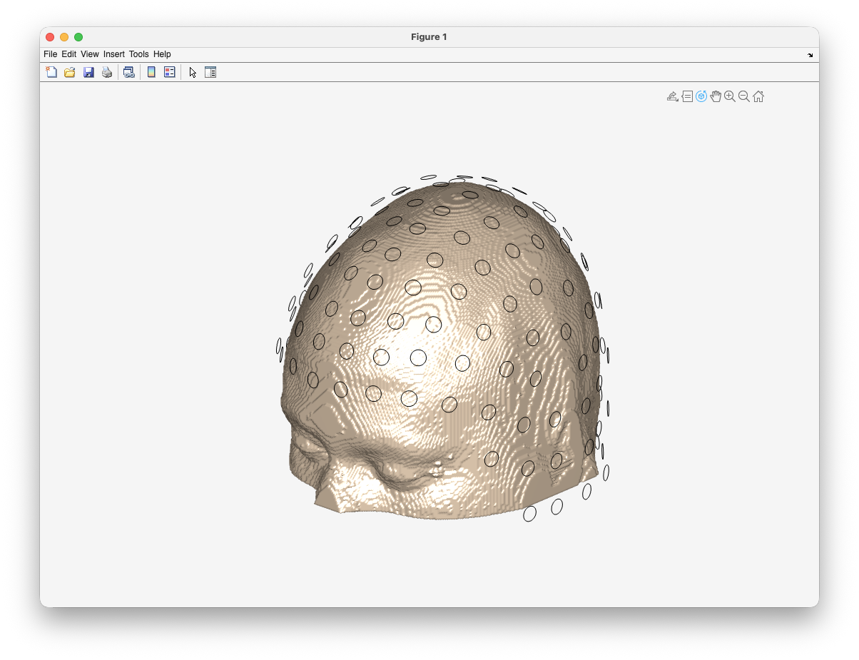
Compared to the CTF systems, you can see that the sensors are much closer to the scalp and hence also to the dipoles on the cortical sheet.

We proceed by computing the leadfield and the sensitivity maps for the FieldLine system.

cfg = [];
cfg.headmodel = headmodel; % singleshell model for MEG
cfg.sourcemodel = sourcemodel; % cortical sheet
cfg.sourcemodel.inside = ones(size(sourcemodel.pos,1), 1);
cfg.orientation = 'yes'; % compute the dipole orientations
cfg.grad = fieldlinebeta2_shifted;
sourcemodel_fieldlinebeta2 = ft_prepare_leadfield(cfg);

cfg = [];
cfg.grad = fieldlinebeta2_shifted;
sensitivity_fieldlinebeta2 = ft_sensitivitymap(cfg, sourcemodel_fieldlinebeta2);

We could now use the same code as above to plot the distance of the dipoles in the sourcemodel to the sensors (which is considerably closer than for the CTF systems) and the relative sensitivities. However, more interesting is to directly compare the OPM sensitivity to that of the 275-channel CTF system.

Compare CTf and OPM sensitivity maps

We can compare the abosolute sensitivity of the CTF275 and FieldLine beta2 side by side.

figure

h1 = subplot(1,2,1); title('ctf275')
ft_plot_headshape(scalp, 'facecolor', 'skin_light', 'facealpha', 0.3)
ft_plot_mesh(sourcemodel, 'vertexcolor', sensitivity_ctf275.fixed * 1e6)
ft_plot_sens(ctf275_aligned, 'edgealpha', 0.3)
ft_colormap('-RdBu') % from red to blue, but then the opposite
colorbar
clim([0 120])

h2 = subplot(1,2,2); title('fieldlinebeta2')
ft_plot_headshape(scalp, 'facecolor', 'skin_light', 'facealpha', 0.3)
ft_plot_mesh(sourcemodel, 'vertexcolor', sensitivity_fieldlinebeta2.fixed * 1e6)
ft_plot_sens(fieldlinebeta2_shifted, 'edgealpha', 0.3, 'fiducial', false)
ft_colormap('-RdBu') % from red to blue, but then the opposite
colorbar
clim([0 120])

linkprop([h1, h2], {'CameraPosition', 'CameraUpVector', 'XLim', 'YLim', 'ZLim'});
view([-90 0])
rotate3d

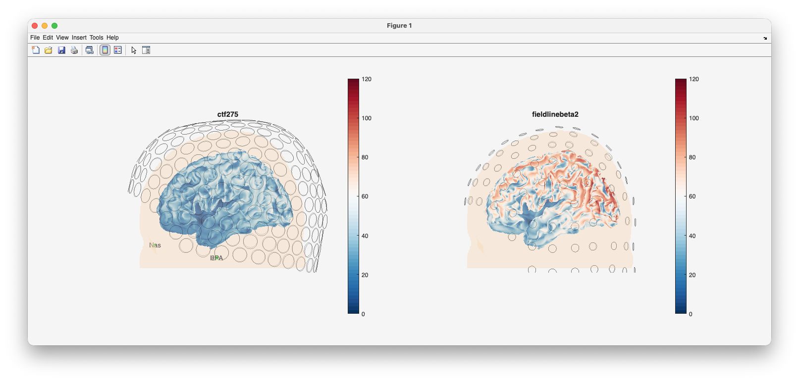
The 275-channel CTF system has a maximum absolute sensitivity of about 60 fT/nAm and with the 144 axial sensors in FieldLine beta2 smart helmet we would obtain a maximum absolute sensitivity of approximately 120 fT/nAm. The FieldLine v3 sensors furthermore allow for recording in the tangential direction, which means that with 144 sensors you can record 288 channels. If we were to take that into account, the sensitivity of the OPM system would be even larger, especially for the superficial dipoles.

However, what we have ignored so far is that the different sensors also have different intrinsic noise characteristics (the OPMs are more noisy) and different sensitivities to the environmental noise (the CTF sensors are axial gradiometers, the OPMs are magnetometers). A full analysis of the signal-to-noise ratio and the effect of the different sensor characteristics and arrangements falls ourtside the scope of this tutorial. The paper by Schoffelen et al (2025) on “Optimal configuration of on-scalp OPMs with fixed channel counts” does a more thorough job and computes the effect that different sensor arrangements have on the sensitivity, also considering sensor noise, environmental noise, and head-movement related noise. The code for those simulations is shared on https://github.com/schoffelen/opm_simulations. Also the paper by Iivanainen et al (2017) on “Measuring MEG closer to the brain: Performance of on-scalp sensor arrays” deals with this.

Summary and conclusion

This tutorial covered how to compute and visualize sensitivity maps for different MEG sensor arrays using an SVD-based approach applied to the leadfield matrix. You have learned how to:

Load an MRI segmentation and cortical sheet source model
Create a singleshell volume conduction model and scalp mesh
Load, align, and preprocess the CTF SQUID sensor arrays
Compute leadfield matrices and sensitivity maps
Visualize distance, free-orientation, and fixed-orientation sensitivity on the cortical surface
Compare sensitivity across different CTF systems (64, 151, 275 channels)
Repeat the analysis for the FieldLine beta2 OPM array, including standoff distance correction

The same procedure can be applied to compare other MEG systems and OPM sensor placements by repeating the leadfield computation and sensitivity analysis for each sensor array. Specifically for OPM systems this approach can also be used to compare the effect of different sensor placements, for example when selecting a subset from the 144 slots in the FieldLine smart helmet, which allows you to optimize the sensor placement for the activity in a specific cortical region.

This tutorial did not deal with the differences in the noise of the individual sensors, or the different sensitivity to environmental noise. It also only consisted of forward solutions of the leadfield matrix given hypothetical sources on the cortical sheet. If you are interested in the influence of the sensitivity and noise differences and/or source reconstruction of real data, you could continue with the beamforming or minimum-norm estimate tutorials.