Beamforming evoked fields and potentials in combined MEG/EEG data
Introduction
In this tutorial we will apply beaforming techniques to event-realted fields. The data used herein has been used and preprocessing procedures have been extensively explained in the Natmeg tutorial dataset. Below we will focus on motor-evoked fields associated with the right-hand button press. We will repeat code to select the trials and preprocess the data as described in the earlier tutorials (trigger-based trial selection, visual artifact rejection). Except, we will focus on motor responses rather than the preceding stimuli. Further, we will compare the measured topography and the corresponding source reconstruction. The quality of the topography often depends on the presence of super-positioned activity of no interest, i.e. ocular and cardiac artifacts. Thus, we will apply ICA in order to identify and subsequently remove such activity.
In this tutorial you will learn about applying beamformer techniques in the time domain. This tutorial further assumes that you made yourself familiar with all the necessary steps such as computing an appropriate head model and lead field matrix, and various options for contrasting the effect of interest against some control/baseline. It is important that you understand the basics of these previous steps explained in the tutorial:natmeg:beamforming.
This tutorial contains the hands-on material of the NatMEG workshop and is complemented by this lecture.
Background
A motor response is typically associated with an event-related field observed over the hemisphere contra lateral to the response hand. The goal of this section is to identify the sources associated with this evoked field. We will apply a beamformer technique. This is a spatially adaptive filter, allowing us to estimate the amount of activity at any given location in the brain. The inverse filter is based on minimizing the source power (or variance) at a given location, subject to ‘unit-gain constraint’. This latter part means that, if a source had power of amplitude 1 and was projected to the sensors by the lead field, the inverse filter applied to the sensors should then reconstruct power of amplitude 1 at that location. Beamforming assumes that sources in different parts of the brain are not temporally correlated. This is key in the context of averaging over trials or in other words computing the most common, thus correlated, feature of the signal. However, “evoked” activity is rarely perfectly correlated over individual observations (trials). Instead it is often characterized by some temporal jitter. This temporal variation will be used here during the computation of the covariance matrix, as such essential for the time-domain beamformer to work.
The brain is divided in a regular three dimensional grid and the source strength for each grid point is computed. The method applied in this example is termed Linearly Constrained Minimum Variance (LCMV) and the estimates are calculated in the time domain (Van Veen et al. 1997). These methods produce a 3D spatial distribution of the power of the neuronal sources. This distribution is then overlaid on a structural image of the subject’s brain. Furthermore, these distributions of source power can be subjected to statistical analysis. It is always ideal to contrast the activity of interest against some control/baseline activity. Options for this will be discussed below, but it is best to keep this in mind when designing your experiment from the start, rather than struggle to find a suitable control/baseline after data collection.
Procedure
To localize the oscillatory sources for the example dataset we will perform the following step
- Reading in the subject specific anatomical MRI using ft_read_mri
- Construct a forward model using ft_volumesegment and ft_prepare_headmodel
- Prepare the source model using ft_prepare_sourcemodel
Next, we head out to investigate the response to the finger movement. We will localize the sources of the motor beta-band activity following the following step
- Load the data from disk and define baseline and poststimulus period using ft_redefinetrial
- Compute the cross-spectral density matrix for all MEG channels using the function ft_freqanalysis
- Compute the lead field matrices using ft_prepare_leadfield
- Compute a common spatial filter and estimate the power of the sources using ft_sourceanalysis
- Compute the condition difference
- Visualize the result with ft_sourceplot
Note that some of the steps will be skipped in this tutorial as we have already done them in the previous days of the workshop.
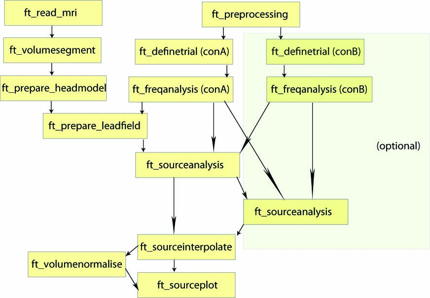
Figure: An example of a pipeline to locate sources associated with evoked fields.
Preparing the data and the forward and inverse model
Loading the data
We will briefly explain the steps that allowed the generation of the epoched file in case you might want to generate the data structure yourself.
The following steps had been performed:
- Defining triggers around which the data will be segmented using ft_definetrial. The data is segmented to include 1.5 seconds prior to trigger onset (i.e. baseline) and 2 second post trigger onset (i.e. response interval).
- Apply some preprocessing such as power line noise removal, demean and detrend using ft_preprocessing
To run the following section of code you need the original dataset oddball1_mc_downsampled.fif and trial function trialfun_oddball_responselocked.m.
clear all
close all

cfg = [];
cfg.dataset = 'oddball1_mc_downsampled.fif';
cfg.channel = 'MEG';

% define trials based on responses
cfg.trialdef.prestim       = 1.5;
cfg.trialdef.poststim      = 2.0;
cfg.trialdef.stim_triggers = [1 2];
cfg.trialdef.rsp_triggers  = [256 4096];
cfg.trialfun               = 'trialfun_oddball_responselocked';
cfg                        = ft_definetrial(cfg);

% preprocess MEG data
cfg.continuous             = 'yes';
cfg.demean                 = 'yes';
cfg.dftfilter              = 'yes';
cfg.dftfreq                = [50 100];

data_meg_clean    = ft_preprocessing(cfg);
The resulting epoched data can be downloaded here and you can load it using the following command:
load data_meg_clean
Next, we perform the independent component analysis according to the following steps:
- Resampling the data to a lower sample rate in order to speed up ICA computation ft_resampledata. Note, that we will compute the ICA twice in order to retain the original sampling rate. The option cfg.resamplefs depends on your knowledge about the spectral characteristics of the artifacts you would like to discover. Vertical and horizontal eye movements are typically dominated by high energy in the low frequency <10 Hz. Therefore everything above the Nyquist frequency of the targeted signal, in this case 20 Hz, is an appropriate sampling rate. Cardiac artifacts vary over the entire frequency spectrum, although there is some dominance in the slower frequencies too. The decision about the new sampling frequency thus strongly depends on your needs. If you are interested in the detection of caridac and oculo-motor activity a sampling rate of >100 Hz will be appropriate for most of the cases.
- Perform the independent components analysis on the resampled data ft_componentanalysis
-
Repeat the independent components analysis on the original data by applying the linear demixing and topography labels form the previous step
% project the cont data thru the components cfg = []; cfg.resamplefs = 140; cfg.detrend = ‘no’; datads = ft_resampledata(cfg, data_meg_clean);
% perform the independent component analysis (i.e., decompose the data) cfg = []; cfg.method = ‘runica’; cfg.runica.maxsteps = 100; comp = ft_componentanalysis(cfg, datads);
cfg = []; cfg.unmixing = comp.unmixing; cfg.topolabel = comp.topolabel; comp_meg=ft_componentanalysis(cfg, data_meg_clean);
Now we could explore the decomposed data by using ft_databrowser
cfg = [];
cfg.channel = {comp_meg.label{1:5}}; % components to be plotted
cfg.layout = 'neuromag306mag.lay'; % specify the layout file that should be used for plotting
cfg.compscale = 'local';

ft_databrowser(cfg, comp_meg);
Take your time to browse and evaluate the topographies and the corresponding time courses. We will reject several of these with ft_rejectcomponent
cfg = [];
cfg.component = [1:6 10 11 15];
data_meg_clean_ica = ft_rejectcomponent(cfg, comp_meg);
Averaging and plotting the response related field
In the first step we re-segment the data into left and right hand responses using the information organized in the trialinfo substructure. We use ft_redefinetrial. After this we’ll focus on right hand responses for simplicity and average over repetitions using ft_timelockanalysis. Finally, we use ft_topoplotER and ft_singleplotER with a predefined latency window to plot the topography and time course of the early motor evoked field.
cfg = [];
cfg.trials    = find(data_meg_clean_ica.trialinfo(:,1) == 256);
data_left     = ft_redefinetrial(cfg, data_meg_clean_ica);

cfg.trials    = find(data_meg_clean_ica.trialinfo(:,1) == 4096);
data_right    = ft_redefinetrial(cfg, data_meg_clean_ica);
%%
tlk = ft_timelockanalysis([],data_right);
%%
cfg = [];
cfg.fontsize = 6;
cfg.layout = 'neuromag306mag.lay';
cfg.xlim = [0.040553 0.062673];
figure;
subplot(2,2,1);ft_topoplotER(cfg, tlk);

cfg.channel = {'MEG0431'}
cfg.xlim    = [-.2 1];
subplot(2,2,2);ft_singleplotER(cfg,tlk);
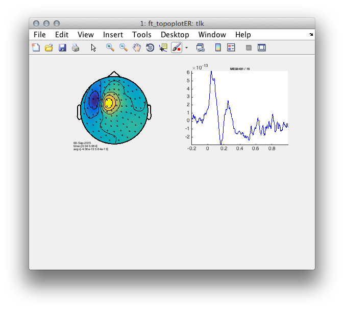
Figure 1: Topography and time course of the motor evoked response performed with the right hand.
Use your knowledge about the distribution of the ingoing and outgoing field.
- What is the orientation of the source?
- Is this source likely located on a gyral bank or sulcal wall? </div>
Loading the headmodel
The first requirement for the source reconstruction procedure is that we need a forward model. The forward model allows us to calculate the distribution of the magnetic field on the MEG sensors given a hypothetical current distribution. We are going to use the forward model that was calculated in the dipole fitting tutorial which you can download to your working directory here.
Load the forward model using the following cod
load headmodel_meg.mat
Computing the leadfield
The next step is to discretize the brain volume into a grid. For each grid point the lead field matrix is calculated. It is calculated with respect to a grid with a 1 cm resolution.
Sensors that were previously removed from the data set should also be removed when calculating the leadfield.
We first prepare the magnetometer and electrode position information from the dataset that can be downloaded here.
dataset = 'oddball1_mc_downsampled.fif';
grad    = ft_read_sens(dataset, 'senstype', 'meg');
elec    = ft_read_sens(dataset, 'senstype', 'eeg');
If you are not contrasting the activity of interest against another condition or baseline time-window, then you may choose to normalize the lead field (cfg.normalize=’yes’), which will help control against the power bias towards the center of the head.
% Create leadfield grid
cfg = [];
cfg.channel    = data_right.label; % ensure that rejected sensors are not present
cfg.grad       = grad;
cfg.headmodel  = headmodel_meg;
cfg.reducerank = 2; % default for MEG is 2, for EEG is 3
cfg.resolution = 1;   % use a 3-D grid with a 1 cm resolution
cfg.unit       = 'cm';
cfg.tight      = 'yes';
[grid] = ft_prepare_leadfield(cfg);
Save the source model with the leadfields:
save grid grid
The grid data structure has the following field
grid =
            xgrid: [-6 -5 -4 -3 -2 -1 0 1 2 3 4 5 6 7]% X-axsis grid
            ygrid: [-8 -7 -6 -5 -4 -3 -2 -1 0 1 2 3 4 5 6 7 8 9]% Y-axis grid
            zgrid: [-4 -3 -2 -1 0 1 2 3 4 5 6 7 8 9]% Z-axis grid
              dim: [14 18 14]                     % Size of the dimensions in the grid
              pos: [3528x3 double]                % 3d coordinates of every position in the grid
             unit: 'cm'                           % Units of the coordinates in the grid
           inside: [3528x1 logical]               % Grid points inside the brain
              cfg: [1x1 struct]                   % Grid points outside the brain
        leadfield: {1x3528 cell}                  % Leadfield for every position in grid
            label: {102x1 cell}                   % Sensor labels
  leadfielddimord: '{pos}_chan_ori'               % Dimord structure of the leadfield
(MEG) Source analysis on motor evoked field
Using the data covariance matrix and the lead field matrices a spatial filter is calculated for each grid point. By applying the filter to the time-domain data we can then estimate the power for the pre- and post-response activity. This results in a power estimate for each grid point. We will focus on right hand responses. First, we select the latencies of the early evoked field and the pre response baselin
cfg = [];
cfg.toilim = [-.15 -.05];
datapre = ft_redefinetrial(cfg, data_right);
cfg.toilim = [.05 .15];
datapost = ft_redefinetrial(cfg, data_right);
We compute the covariance matrix during the call to ft_timelockanalysis. Note that the data covariance matrix is computed on the entire interval including the pre and post-response latencies. This approach is similar to the common filter minimizing the influence of different spatial leakage profiles of the pre and post-response spatial filters.
cfg = [];
cfg.covariance = 'yes';
cfg.covariancewindow = [-.15 .15];
avg = ft_timelockanalysis(cfg, data_right);

cfg = [];
cfg.covariance = 'yes';
avgpre = ft_timelockanalysis(cfg, datapre);
avgpst = ft_timelockanalysis(cfg, datapost);
Now using the headmodel and the precomputed leadfield we make three subsequent calls to ft_sourceanalysis. First we compute one spatial filter per location (e.g., voxel) on the basis of the entire latency interval of pre and post-response data. Specifying the cfg.keepfilter = 'yes' allows for a subsequent application of the spatial filters to the pre- and post-response data separately. The purpose of lambda is discussed in Exercise 6. By using cfg.keepfilter = 'yes' we let ft_sourceanalysis return the filter matrix in the source structure.
%% first call to ft_sourceanalysis keeping the spatial filters
cfg = [];
cfg.method = 'lcmv';
cfg.grid = grid;
cfg.headmodel = headmodel_meg;
cfg.lcmv.keepfilter = 'yes';
cfg.lcmv.lambda = '5%';
cfg.channel = {'MEG'};
cfg.senstype = 'MEG';
sourceavg = ft_sourceanalysis(cfg, avg);

%% second and third call to ft_sourceanalysis now applying the precomputed filters to pre and %post intervals
cfg = [];
cfg.method = 'lcmv';
cfg.grid = grid;
cfg.sourcemodel.filter = sourceavg.avg.filter;
cfg.headmodel = headmodel_meg;
sourcepreM1 = ft_sourceanalysis(cfg, avgpre);
sourcepstM1 = ft_sourceanalysis(cfg, avgpst);
The source data structure has the following fields:
sourceavg =
    time: [1x876 double]   % time dimension of the input data
     dim: [14 18 14]       % 3D dimensions of the scanned space
  inside: [3528x1 logical] % locations inside the brain
     pos: [3528x3 double]  % locations outside the brain
  method: 'average'        % mean power over repetitions
     avg: [1x1 struct]     % subfield containing power, dipole moments and spatial filters at each location
     cfg: [1x1 struct]     % configuration options used during the call to ft_sourceanalysis
Plotting sources of response related evoked field
The strategy around circumventing the noise bias towards the center of the head has been addressed and the bias itself has been illustrated here. Here we will contrast the estimated source power of the response interval against the one from the pre-response.
M1=sourcepstM1;
M1.avg.pow=(sourcepstM1.avg.pow-sourcepreM1.avg.pow)./sourcepreM1.avg.pow;
The grid of estimated power values can be plotted superimposed on the anatomical MRI. This requires the output of ft_sourceanalysis to match position of the MRI. The function ft_sourceinterpolate aligns the source level activity with the structural MRI. We only need to specify what parameter we want to interpolate and to specify the MRI we want to use for interpolation.
First we will load the MRI. It is important that you use the MRI realigned with the sensor or your source activity data will not match the anatomical data. We will load the realigned MRI from the dipole fitting tutorial which can be downloaded to the working directory here.
load mri_segmented.mat
Subsequently, we interpolate the source power onto the individual MRI.
cfg              = [];
cfg.voxelcoord   = 'no';
cfg.parameter    = 'avg.pow';
cfg.interpmethod = 'nearest';
source_int  = ft_sourceinterpolate(cfg, M1, mri_segmented);
After which, we can plot the interpolated data. In order to emphasize “the hill” of activity we are interested in, we create a mask that in the present case highlights 30 % of the total activity. Note, that this threshold is arbitrary and is mainly used for illustrative purposes. An alternative to this is provided below.
source_int.mask = source_int.pow > max(source_int.pow(:))*.3; % 30 % of maximum
cfg               = [];
cfg.method        = 'ortho';
cfg.funparameter  = 'pow';
cfg.maskparameter = 'mask';
cfg.location = [-42 -18 67];
cfg.funcolormap = 'jet';
ft_sourceplot(cfg, source_int);
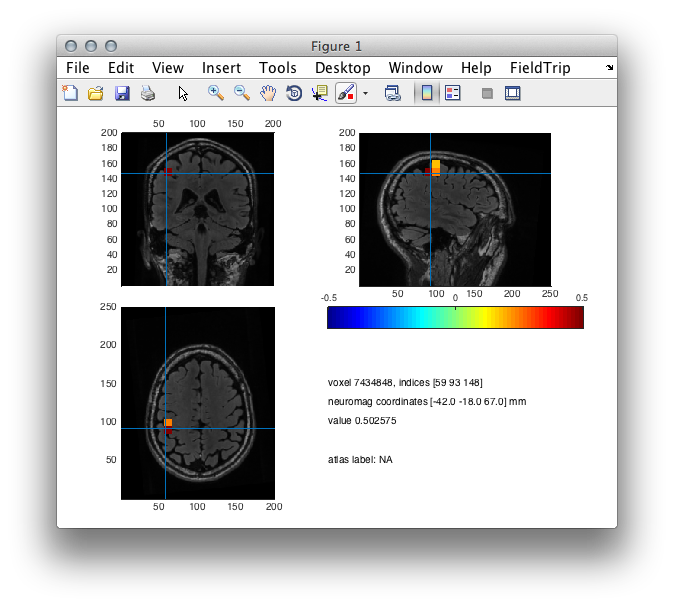
Figure 2: A source plot of the motor evoked field- ratio between the pre- and post-response conditions.
The ‘ortho’ method is not the only plotting method implemented. Use the ‘help’ of ft_sourceplot to find what other methods there are and plot the source level results. What are the benefits and drawbacks of these plotting routines?
Exercise: determining anatomical labels
If you were to name the anatomical label of the source of this motor beta, what you say? What plotting method is most appropriate for this?
With the use of cfg.atlas you can specify a lookup atlas, which ft_sourceplot will use to return appropriate anatomical labels. One for the MNI template is distributed with FieldTrip and can be found in ‘fieldtrip/template/atlas/aal/ROI_MNI_V4.nii’. Be aware that for this to work you need to realign your anatomical and functional data into MNI coordinates. An example how to achieve this is to align the leadfield grid of the individual subject to a leadfield grid in MNI space.
Exercise: regularization
The regularization parameter was lambda = ‘5%’. Change it to ‘0%’ or to ‘10%’ and plot the power estimate. How does the regularization parameter affect the properties of the spatial filter?
Exercise: covariance matrix computation
The covariance matrix was computed on the basis of the single trials. Compute the cov matrix on the basis of the mean over the trials and redo the steps above. Why and how is the source reconstructed power changed?
(MEG) Plotting sources of response related evoked field using statistical threshold
In the previous step we applied an arbitrary chosen threshold for plotting the data. It is also possible to apply the permutation framework as extensively described in the statistic tutorials. It is strongly recommended to make yourself familiar with the framework and consult also the on-line lecture.
This tutorial contains the hands-on material of the NatMEG workshop and is complemented by this lecture.
First we will repeat some of the previous steps. We will compute the covariance matrix on the basis of the data including the pre and post-response latencies. This is followed by averaging of the pre and post data segments separately, yet keeping the individual observations using the option cfg.keeptrials = ‘yes’. Here it is important that we also calculate the single-trial covariance using the option cfg.covariance = ‘yes’ as this will later be used to calculate the source activity.
If this is where you started in the tutorial, make sure you have downloaded and loaded the necessary data: headmodel_meg.mat, datapre.mat, datapost.mat, grid.mat, data_right.mat
% load the data
load headmodel_meg
load datapre
load datapost
load grid
load data_right

cfg = [];
cfg.covariance='yes';
cfg.covariancewindow = [-.15 .15];
avg = ft_timelockanalysis(cfg,data_right);

cfg = [];
cfg.keeptrials = 'yes';
cfg.covariance = 'yes'; % This is important as the single-trial source activity is calculated based on the covariance matrix
avgpre = ft_timelockanalysis(cfg,datapre);
avgpst = ft_timelockanalysis(cfg,datapost);
Next, we repeat the three subsequent calls to ft_sourceanalysis. The first computes the spatial filters much in the same way demonstrated above. Because of low signal-to-noise ratio on single trial level it is not recommended to compute them on individual trials. Subsequently, single trial source power estimates are kept in the output structure by specifying cfg.rawtrial = 'yes'.
cfg=[];
cfg.method = 'lcmv';
cfg.grid = grid;
cfg.headmodel = headmodel_meg;
cfg.lcmv.keepfilter = 'yes';
cfg.lcmv.lambda = '5%';
cfg.channel = {'MEG'};
sourceavg = ft_sourceanalysis(cfg, avg);

cfg = [];
cfg.method = 'lcmv';
cfg.grid = grid;
cfg.sourcemodel.filter = sourceavg.avg.filter;
cfg.rawtrial = 'yes';
cfg.headmodel = headmodel_meg;
sourcepreM1 = ft_sourceanalysis(cfg, avgpre);
sourcepstM1 = ft_sourceanalysis(cfg, avgpst);
The source structure now contains the single trial estimates in the field sourcepstM1.trial
sourcepstM1 =
    time: [1x26 double]
     dim: [14 18 14]
  filter: {3528x1 cell}
  inside: [3528x1 logical]
     pos: [3528x3 double]
  method: 'rawtrial'
   trial: [1x50 struct]
      df: 50
     cfg: [1x1 struct]
Now we can statistically compare the difference between the pre and post response source power using ft_sourcestatistics and plot the output after interpolating onto the anatomical image with ft_sourceinterpolate.
cfg = [];
cfg.parameter        = 'pow';
cfg.dim              = grid.dim;
cfg.method           = 'montecarlo';
cfg.statistic        = 'ft_statfun_depsamplesT';
cfg.correctm         = 'cluster';
cfg.clusteralpha     = 0.05;
cfg.clusterstatistic = 'maxsum';
cfg.tail             = 0;
cfg.clustertail      = 0;
cfg.alpha            = 0.025;
cfg.numrandomization = 10000;

ntrials = numel(sourcepreM1.trial);
design  = zeros(2,2*ntrials);
design(1,1:ntrials) = 1;
design(1,ntrials+1:2*ntrials) = 2;
design(2,1:ntrials) = [1:ntrials];
design(2,ntrials+1:2*ntrials) = [1:ntrials];

cfg.design   = design;
cfg.ivar     = 1;
cfg.uvar     = 2;
stat = ft_sourcestatistics(cfg,sourcepstM1,sourcepreM1);
Note, we make two subsequent calls to ft_sourceinterpolate. One for the functional data (e.g., t-value distribution) and the other for a binary mask of 0 and 1 indexing voxels of significant condition differences.
cfg              = [];
cfg.voxelcoord   = 'no';
cfg.interpmethod = 'nearest';
cfg.parameter    = 'stat';
statint = ft_sourceinterpolate(cfg, stat, mri_segmented);
cfg.parameter    = 'mask';
maskint = ft_sourceinterpolate(cfg, stat, mri_segmented);
statint.mask = maskint.mask;
Finally, we plot the result. Instead of ratio the functional data is now represented in t-values.
cfg               = [];
cfg.method        = 'ortho';
cfg.funparameter  = 'stat';
% cfg.maskparameter = 'mask';
cfg.location = [-42 -18 67];
cfg.funcolormap = 'jet';
ft_sourceplot(cfg,statint);

Figure 3: A source plot of the difference between the pre- and post-response conditions expressed in t-values.
Exercise: discuss and evaluate the spm map
Uncomment the option cfg.maskparameter = ‘mask’; and try to interpret what you see. Consider the scalp topography too. In the context of the present question ‘Whereare the generators of the MEP?’ is there a favorable thresholding approach? If so, why?
(MEG) Reconstructing the time course of activity in the primary motor cortex
The ultimate motivation of source analysis of M/EEG data is the reconstruction of the time course of the neural activity at a particular location. The following section will demonstrate how to achieve this. First we have to compute a leadfield at the desired location (e.g., M1 identified in the previous steps) using ft_prepare_leadfield. The only difference to the previous leadfield computation is that instead of discretizing the brain into multiple grid locations we now focus only on the location within the primary motor cortex. Next, we repeat the above steps, i.e. covariance matrix computation using ft_timelockanalysis and ft_sourceanalysis. Finally, we will multiply the data consisting the single trial observations with the spatial filters at the desired location. This is commonly known as virtual sensor computation and has been also covered in the virtual sensors tutorial in the context of different task demands.
Compute leadfield at desired location
cfg = [];
cfg.headmodel = headmodel_meg;
cfg.channel = data_right.label;
cfg.sourcemodel.pos = [-42 -18 67]./10; % units of cm
cfg.grad = grad;
cfg.unit = 'cm';
sourcemodel_virt = ft_prepare_leadfield(cfg);
Compute the covariance matrix
cfg = [];
cfg.channel = data_right.label;
cfg.covariance = 'yes';
cfg.covariancewindow = [.05 .18];
avg = ft_timelockanalysis(cfg,data_right);
Perform source analysis
cfg = [];
cfg.method = 'lcmv';
cfg.grid = sourcemodel_virt;
cfg.headmodel = headmodel_meg;
cfg.lcmv.keepfilter = 'yes'; % keep filters in the output, which are later multiplied with the data
cfg.lcmv.fixedori ='yes'; % consider only the dominant orientation
cfg.lcmv.lamda = '5%';
source = ft_sourceanalysis(cfg, avg);
Multiply filters with the data and organize into FieldTrip sensible data structure
spatialfilter = cat(1,source.avg.filter{:});
virtsens = [];
for i=1:length(data_right.trial)
  virtsens.trial{i} = spatialfilter*data_right.trial{i};
end
virtsens.time = data_right.time;
virtsens.fsample = data_right.fsample;
virtsens.label = {'M1'}';
Now we will use ft_timelockanalysis and ft_freqanalysis in order to evaluate the result by plotting it with ft_singleplotER and ft_singleplotTFR respectively. Note, all the details around event-related averaging and time-frequency analysis are covered by the the event-related fields tutorial and the time-frequency tutorial. It is recommended that you are familiar with these before you continue.
%% compute the event-related average at location M1
cfg = [];
cfg.preproc.hpfilter = 'yes';
cfg.preproc.hpfreq = 1;
cfg.preproc.lpfilter = 'yes';
cfg.preproc.lpfreq = 40;
tlkvc = ft_timelockanalysis(cfg, virtsens);

%% compute the time-frequency representation of power (TFR)at location M1
cfg            = [];
cfg.output     = 'pow';
cfg.method     = 'mtmconvol';
cfg.taper      = 'hanning';
cfg.foi        = 1:1:40;
cfg.t_ftimwin  = ones(length(cfg.foi),1).*0.5;
cfg.toi        = -.5:0.05:1.75;
cfg.keeptrials = 'no';
tfrvc= ft_freqanalysis(cfg,virtsens);

% baseline correction
cfg = [];
cfg.baseline = [-.5 0];
cfg.baselinetype = 'db';
tfrvcbl = ft_freqbaseline(cfg, tfrvc);
Now we can plot the result.
figure;
for i=1:length(tlkvc.label)
  cfg = [];
  cfg.channel   = tlkvc.label{i};
  cfg.parameter = 'avg';
  cfg.xlim      = [-.3 1.75];

  subplot(2,2,i); ft_singleplotER(cfg, tlkvc);
end
for i=1:length(tfrvc.label)
  cfg = [];
  cfg.channel = tfrvc.label{i};
  cfg.zlim    = [-3 3];
  cfg.xlim    = [-.5 2];
  cfg.ylim    = [1 40];
  subplot(2,2,i+1); ft_singleplotTFR(cfg, tfrvcbl);
end
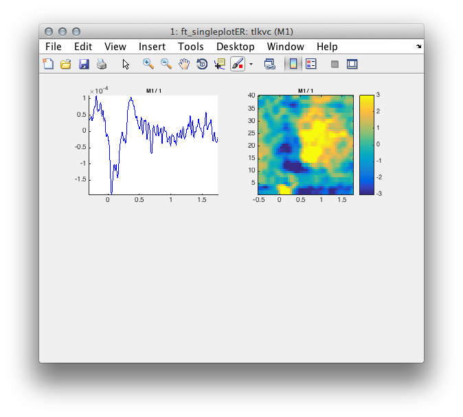
Figure 4: Time course of activity in the primary motor cortex averaged across trials (left) and its single trial time-frequency decomposition right.
Exercise: evoked vs. induced activity
Take your time to verbalize what you see. Try to decompose the averaged response into the time-frequency domain. Plot the result with and without baseline correction. Why is there a difference?
(EEG) The forward model and lead field matrix
We will continue to analyze the EEG data according to a series of steps similar to the MEG. Try to note the differences between analyzing the EEG and MEG data. The data used in this tutorial can be downloaded here.
load data_eeg_reref_ica
%% sort into left and right hand response
cfg = [];
cfg.trials = find(data_eeg_reref_ica.trialinfo(:,1) == 256);
data_eeg_left = ft_redefinetrial(cfg, data_eeg_reref_ica);

cfg.trials = find(data_eeg_reref_ica.trialinfo(:,1) == 4096);
data_eeg_right = ft_redefinetrial(cfg, data_eeg_reref_ica);
Prepare data for source analysis
cfg = [];
cfg.toilim = [-.15 -.05];
datapre = ft_redefinetrial(cfg, data_eeg_right);
cfg.toilim = [.05 .15];
datapost = ft_redefinetrial(cfg, data_eeg_right);

%% output cov matrix of the entire interval
cfg = [];
cfg.covariance='yes';
cfg.covariancewindow = [-.15 .15];
avg = ft_timelockanalysis(cfg,data_eeg_right);
cfg = [];
cfg.covariance='yes';
avgpre = ft_timelockanalysis(cfg, datapre);
avgpst = ft_timelockanalysis(cfg, datapost);
EEG head model & data
As before, we will use the head model calculated in the dipole fitting tutorial and the preprocessed data in order to compute the leadfield.
Load the EEG head model using the following code:
load headmodel_eeg.mat
(EEG) Lead field calculation
The leadfield is calculated using ft_prepare_leadfield.
cfg = [];
cfg.elec       = elec;
cfg.channel    = data_eeg_reref_ica.label;
cfg.headmodel  = headmodel_eeg;
cfg.reducerank = 3; % default for MEG is 2, for EEG is 3
cfg.resolution = 1;   % use a 3-D grid with a 1 cm resolution
cfg.unit       = 'cm';
cfg.tight      = 'yes';
[grid] = ft_prepare_leadfield(cfg);
save grid_eeg grid
Discuss the option cfg.lcmv.reducerank = 3
(EEG) Source analysis
Now that we have everything prepared we can start to calculate the spatial filter through which we we project the data from both conditions.
cfg=[];
cfg.method='lcmv';
cfg.grid=grid;
cfg.elec = elec;
cfg.headmodel=headmodel_eeg;
cfg.lcmv.keepfilter='yes';
cfg.lcmv.lambda = '5%';
cfg.channel           = data_eeg_reref_ica.label;
cfg.senstype = 'EEG';
sourceavg=ft_sourceanalysis(cfg, avg);

%%
cfg=[];
cfg.method='lcmv';
cfg.elec = elec;
cfg.grid=grid;
cfg.sourcemodel.filter=sourceavg.avg.filter;
cfg.headmodel=headmodel_eeg;
cfg.lcmv.lambda = '5%';
cfg.channel           = data_eeg_reref_ica.label;
cfg.senstype = 'EEG';
sourcepreM1=ft_sourceanalysis(cfg, avgpre);
sourcepstM1=ft_sourceanalysis(cfg, avgpst);
Again we express the source power as relative change to the pre response interval
M1eeg=sourcepstM1;
M1eeg.avg.pow=(sourcepstM1.avg.pow-sourcepreM1.avg.pow)./sourcepreM1.avg.pow;
And interpolate the result onto the anatomical MRI.
cfg              = [];
cfg.voxelcoord   = 'no';
cfg.parameter    = 'pow';
cfg.interpmethod = 'nearest';
source_int  = ft_sourceinterpolate(cfg, M1eeg, mri_segmented);
Finally, we can plot the result using the same masking strategy as in the MEG section
source_int.mask = source_int.pow > max(source_int.pow(:))*.3; % 50 % of maximum
cfg               = [];
cfg.method        = 'ortho';
cfg.funparameter  = 'pow';
cfg.maskparameter = 'mask';
cfg.location = [-28 -17 67];
cfg.funcolorlim = [-.2 .2];
cfg.funcolormap = 'jet';
ft_sourceplot(cfg,source_int);
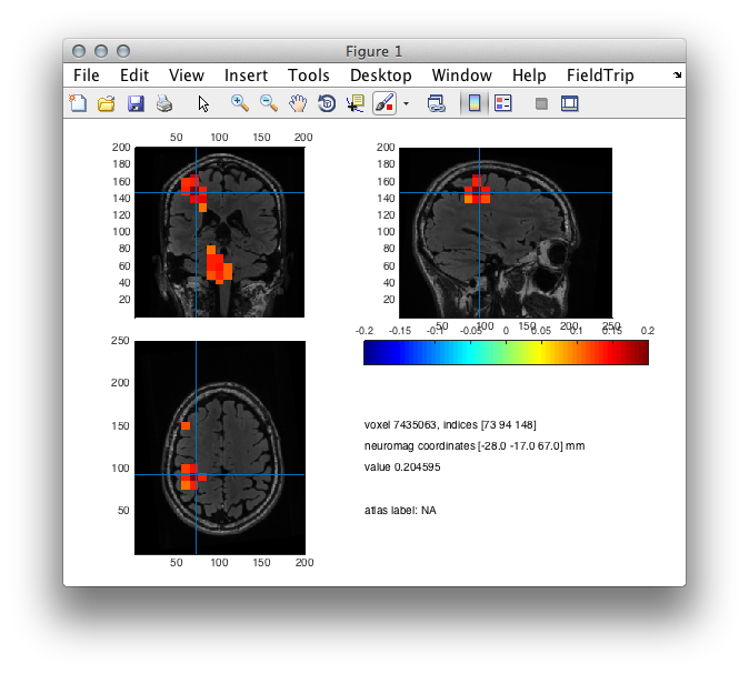
Figure 5: Source plot of reconstructed activity using EEG.
We would like to compare the time course of activity reconstructed with MEG and EEG. Therefore we repeat the above virtual sensor analysis and plot the MEG and EEG result back-to-back.
Compute leadfield at location M1
cfg=[];
cfg.headmodel=headmodel_eeg;
cfg.channel           = data_eeg_reref_ica.label;
cfg.sourcemodel.pos=[-28 -17 67]./10; % units of cm
cfg.elec = elec;
cfg.unit = 'cm';
sourcemodel_virt=ft_prepare_leadfield(cfg);
Source reconstruction
cfg = [];
cfg.channel=data_eeg_right.label;
cfg.covariance='yes';
cfg.covariancewindow=[.05 .18];
avg = ft_timelockanalysis(cfg,data_eeg_right);

cfg=[];
cfg.method='lcmv';
cfg.senstype = 'EEG';
cfg.channel=data_eeg_right.label;
cfg.elec = elec;
cfg.grid = sourcemodel_virt;
cfg.headmodel=headmodel_eeg;
cfg.lcmv.keepfilter='yes';
cfg.lcmv.fixedori='yes';
cfg.lcmv.lamda='5%';
source=ft_sourceanalysis(cfg, avg);
Multiply filters with data
spatialfilter=cat(1,source.avg.filter{:});
virtsens=[];
for i=1:length(data_eeg_right.trial)
  virtsens.trial{i}=spatialfilter*data_eeg_right.trial{i};
end
virtsens.time=data_eeg_right.time;
virtsens.fsample=data_eeg_right.fsample;
virtsens.label={'M1'}';
Perform event-related averaging and time-frequency analysis
cfg=[];
cfg.preproc.hpfilter='yes';
cfg.preproc.hpfreq=1;
cfg.preproc.lpfilter='yes';
cfg.preproc.lpfreq=40;
tlkvc=ft_timelockanalysis(cfg, virtsens);

cfg              = [];
cfg.output       = 'pow';
cfg.method       = 'mtmconvol';
cfg.taper        = 'hanning';
cfg.foi          = 1:1:40;
cfg.t_ftimwin    = ones(length(cfg.foi),1).*0.5;
cfg.toi          = -.5:0.05:1.75;
cfg.keeptrials ='no';
tfrvc= ft_freqanalysis(cfg,virtsens);

%% baseline correction
cfg=[];
cfg.baseline=[-.5 0];
cfg.baselinetype='db';
tfrvcbl = ft_freqbaseline(cfg, tfrvc);
Plot the result
figure;
for i=1:length(tlkvc.label)
  cfg=[];
  cfg.channel = tlkvc.label{i};
  cfg.parameter = 'avg';
  cfg.xlim    = [-.3 1.75];

  subplot(2,2,i);ft_singleplotER(cfg,tlkvc);
end
for i=1:length(tfrvc.label)
  cfg=[];
  cfg.channel = tfrvc.label{i};
  cfg.zlim    = [-3 3];
  cfg.xlim    = [-.5 1.75];
  cfg.ylim    = [1 40];
  subplot(2,2,i+1);ft_singleplotTFR(cfg,tfrvcbl);
end
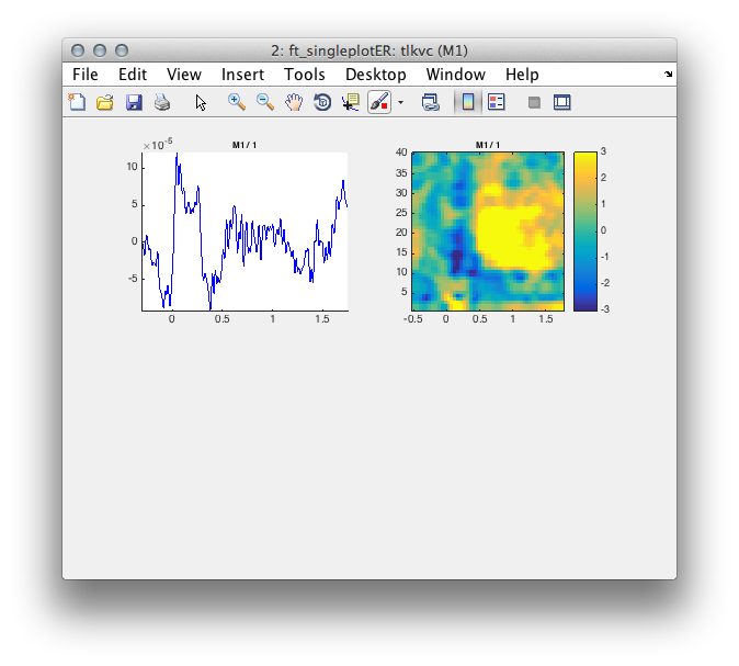
Figure 6: Time course of activity in the primary motor cortex reconstructed with EEG.
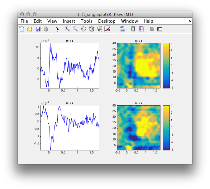
Figure 6: Comparison of time course reconstruction of activity in the primary motor cortex using EEG (top row) and MEG (bottom row).
Summary and suggested further reading
Beamforming source analysis in the time domain with DICS on EEG and MEG data has been demonstrated. Options at each stage and their influence on the results were discussed, such as computing the covariance matrix on the basis of single trials vs. ERF/ERP. The results were plotted on an orthogonal view. Thresholding of the source maps was demonstrated on the basis of an arbitrary and statistical threshold. Finally, virtual sensor time-courses were extracted and compared between the imaging modalities.
Computing event-related fields with MNE or frequency domain beamformer DICS might be of interest. More information on common filters can be found here. If you are doing a group study where you want the grid points to be the same over all subjects, see here. See here for source statistics.
See also the following FAQs:
- Where is the anterior commissure?
- Can I do combined EEG and MEG source reconstruction?
- Can I restrict the source reconstruction to the grey matter?
- How are the different head and MRI coordinate systems defined?
- How are the Left and Right Pre-Auricular (LPA and RPA) points defined?
- How can I check whether the grid that I have is aligned to the segmented volume and to the sensor gradiometer?
- How can I determine the anatomical label of a source or electrode?
- How can I fine-tune my BEM volume conduction model?
- How can I visualize the different geometrical objects that are needed for forward and inverse computations?
- How to coregister an anatomical MRI with the gradiometer or electrode positions?
- Is it good or bad to have dipole locations outside of the brain for which the source reconstruction is computed?
- Is it important to have accurate measurements of electrode locations for EEG source reconstruction?
- What is the conductivity of the brain, CSF, skull and skin tissue?
- What kind of volume conduction models of the head (head models) are implemented?
- Where can I find the dipoli command-line executable?
- Why is there a rim around the brain for which the source reconstruction is not computed?
- Why should I use an average reference for EEG source reconstruction?
See also the following example scripts:
- Combined EEG and MEG source reconstruction
- Common filters in beamforming
- Compute forward simulated data using ft_dipolesimulation
- Compute forward simulated data and apply a beamformer scan
- Compute forward simulated data and apply a dipole fit
- Compute forward simulated data with the low-level ft_compute_leadfield
- Check the quality of the anatomical coregistration
- Localizing the sources underlying the difference in event-related fields
- Fit a dipole to the tactile ERF after mechanical stimulation
- Align EEG electrode positions to BEM headmodel
- How to create a head model if you do not have an individual MRI
- How to import data from MNE-Python and FreeSurfer
- Make leadfields using different headmodels
- Plotting the result of source reconstruction on a cortical mesh
- Source statistics
- Create MNI-aligned grids in individual head-space
- Symmetric dipole pairs for beamforming
- Testing BEM created EEG lead fields
- Use your own forward leadfield model in an inverse beamformer computation