workshop / hangzhou2026 / acquisition /
Planning the acquisition of OPM-MEG data
Introduction
OPMs allow for flexible placement of sensors close to or directly on the scalp. Contrary to SQUID systems, OPM systems do not require a fixed helmet full of sensors. Since OPMs allow for this flexibility, many labs are experimenting with a relatively small number of OPM sensors. Whereas a full-head MEG system has the sensors distributed evenly around the whole head, with a small OPM system you can and should consider what the most optimal placement of the few channels is that you have available.
In this hands-on session we plan the acquisition of OPM-MEG data. We do not record any actual data, but we design the measurement setup: we make a head model of the (template) participant, design an OPM helmet with sensors at the positions of the extended 10-20 system, select a subset of the sensor positions corresponding to the number of OPMs that is available, and compute and plot the sensitivity of the resulting sensor array. The sensitivity map shows which brain regions the sensor array is sensitive to, and hence which placement of a small set of OPM sensors best matches your research question.
Background
This tutorial is a shortened version of the tutorial on designing a custom 3D printed OPM helmet, and combines it with the example on selecting a subset of OPM sensor positions. The figures in this tutorial were generated by running the code, and you will make the same figures on your own computer.
Install and start FieldTrip
If you have not yet done so, install FieldTrip and start it with
restoredefaultpath
cd path_to_directory/fieldtrip-xxxxxxxx
addpath(pwd)
ft_defaults
The code below uses the ft_version function to determine where you installed fieldtrip, so that it works regardless of whether you installed it either in the directory fieldtrip, or in fieldtrip-xxxxxxxx (where xxxxxxxx is the year, month and day) or in fieldtrip-20260812 or so.
The dataset used in this tutorial
We use the standard colin27 template MRI that is included with FieldTrip. All procedures work in exactly the same way with an individual anatomical MRI of your own individual participant, with the main difference that the individual MRI then needs to be read in and the anatomical landmarks need to be determined.
Download the sensor model
The anatomical MRI and cortical sheet are included in the fieldtrip/template directory. The 3D model of the FieldLine OPM sensor is not included with FieldTrip, but can be downloaded from the download server. Download the stl files and place them jointly in a directory, for example on your Desktop. The STL models are needed for planning the OPM sensor placement; the sensor positions and orientations for the analysis are contained in the grad_xyz structure that we will construct further on.
Procedure
The hands-on session covers the following steps
- reading and visualizing an anatomical MRI with ft_read_mri and ft_sourceplot
- segmenting the anatomical MRI with ft_volumesegment
- making a mesh of the head surface with ft_prepare_mesh
- visualize the head surface mesh together with the cortical sheet and anatomical labeling, using ft_read_headshape and ft_read_atlas
- making an individual OPM helmet and placing OPM sensors according to the 10-20 system with ft_electrodeplacement and ft_sensorplacement
- selecting a subset of OPM sensors with ft_electrodeselection and compute sensitivity maps with ft_prepare_leadfield
Processing the anatomical MRI
Reading and visualizing the anatomical MRI
We read the colin27 template MRI, which is a high-quality average MRI of a single person’s brain, created by combining 27 scans of the same individual and aligning them to the MNI152 atlas. This is a widely used template, among others in SPM, and many anatomical atlasses can be combined with it.
[ftver, ftpath] = ft_version;
mri = ft_read_mri(fullfile(ftpath, 'template/anatomy/single_subj_T1_1mm.nii'));
mri.coordsys = 'mni';
The resulting mri structure contains the anatomical volume together with the geometrical transformation between voxel and head coordinates, and the specification of the coordinate system and the units. The coordinate system of this template is spm, which is equivalent to the MNI coordinate system, and the units are in mm. You can inspect the data with ft_determine_coordsys.
We can visualize the anatomy in the standard three orthogonal slices with ft_sourceplot.
figure
cfg = [];
cfg.method = 'ortho';
ft_sourceplot(cfg, mri);

Segmenting the anatomical MRI
For the head surface we need to segment the anatomy, i.e. to determine for every voxel whether it belongs to the head or not. We use ft_volumesegment and ask for the scalp (and all tissues underneath).
cfg = [];
cfg.output = 'scalp';
mri_segmented = ft_volumesegment(cfg, mri);

% we can keep the original anatomy
mri_segmented.anatomy = mri.anatomy;
The result is a structure with a binary scalp field. We can visualize it with ft_sourceplot, plotting the scalp segmentation as the “functional” parameter on top of the anatomy.
figure
cfg = [];
cfg.method = 'ortho';
cfg.funparameter = 'scalp';
cfg.funcolormap = 'jet';
ft_sourceplot(cfg, mri_segmented);
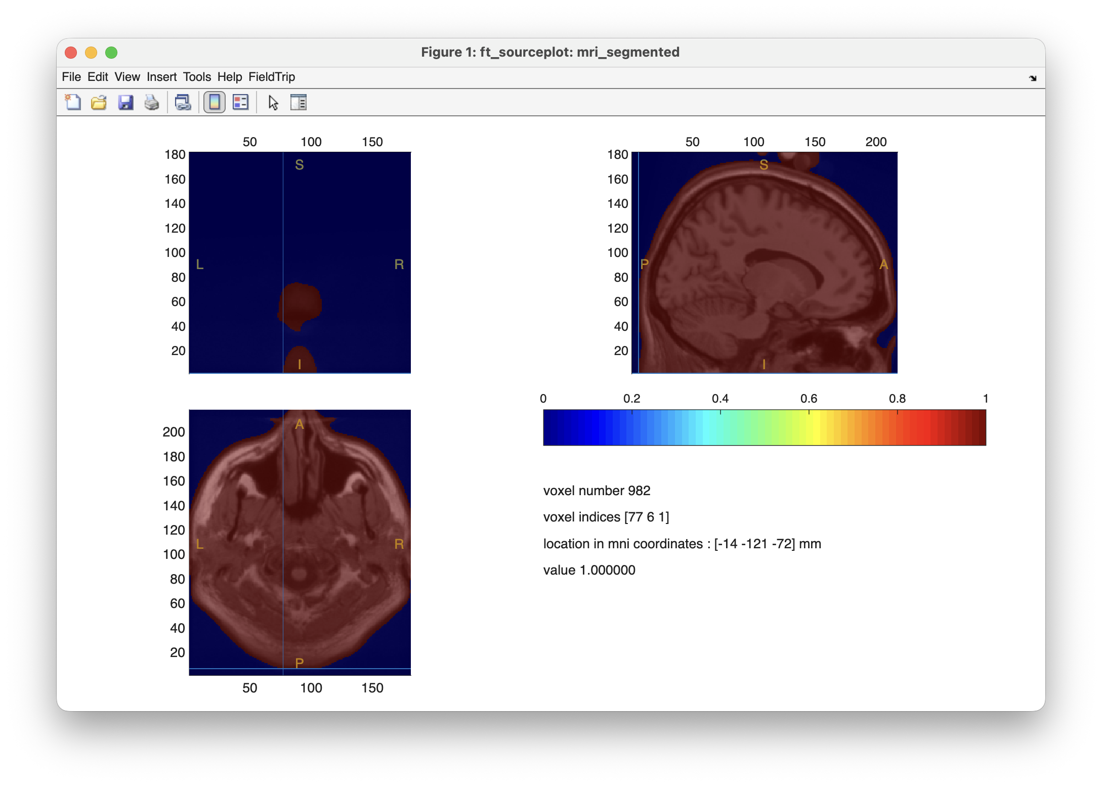
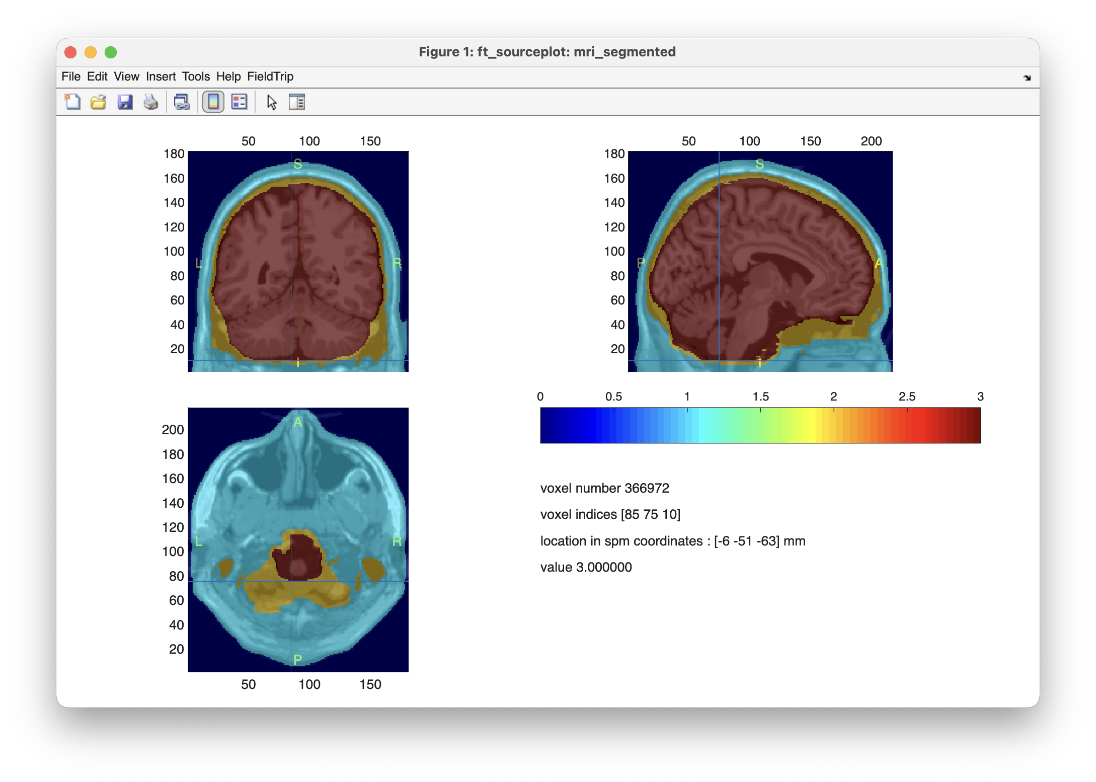
The original colin27 template MRI has a sort of bar at the top of the head which complicates the segmentation. Hence we will proceed with a precomputed segmentation in which the bar has been removed. This also includes the brain and skull.
[ftver, ftpath] = ft_version;
mri_segmented = ft_read_mri(fullfile(ftpath, 'template/headmodel/standard_seg.mat'));
mri_segmented.seglabel = {'scalp', 'skull', 'brain'}; % this was actually determined in the following figure

figure
cfg = [];
cfg.method = 'ortho';
cfg.funparameter = 'seg'; % it is now called "seg"
cfg.funcolormap = 'jet';
ft_sourceplot(cfg, mri_segmented);
Making a mesh of the head surface
We now construct a surface mesh that describes the outer surface of the scalp. This mesh serves both as the head shape for the sensor placement and as the basis for the helmet. We use ft_prepare_mesh with the projectmesh method, which gives a mesh with a specified number of vertices that is as smooth as possible.
cfg = [];
cfg.method = 'projectmesh';
cfg.numvertices = 4000;
cfg.tissue = 'scalp';
headshape = ft_prepare_mesh(cfg, mri_segmented);
We plot the head surface mesh.
figure
ft_plot_headshape(headshape, 'facecolor', 'skin', 'facealpha', 0.8, 'edgecolor', [0.5 0.5 0.5]);
ft_headlight
view([90 0])

Visualize the head with the cortex and atlas labels
To relate the sensor positions to the underlying brain anatomy, we also need the cortical surface. For this we could use FreeSurfer, but as that takes a lot of time to run, here we continue with a decimated version of the cortical surface with 20484 vertices, which we read with ft_read_headshape.
[ftver, ftpath] = ft_version;
cortex = ft_read_headshape(fullfile(ftpath, 'template/sourcemodel/cortex_20484.surf.gii'));
cortex = ft_convert_units(cortex, 'mm');
To color the cortex with anatomical labels, we use the Automated Anatomical Labeling (AAL) atlas, which is included as a template atlas in FieldTrip.
[ftver, ftpath] = ft_version;
atlas = ft_read_atlas(fullfile(ftpath, 'template/atlas/aal/ROI_MNI_V4.nii'));
The atlas is a volumetric segmentation in MNI coordinates with 116 different tissue labels. You can plot the color-coded regions with the following code:
figure
cfg = [];
cfg.funparameter = 'tissue';
cfg.funcolormap = 'jet';
cfg.atlas = atlas;
ft_sourceplot(cfg, atlas);
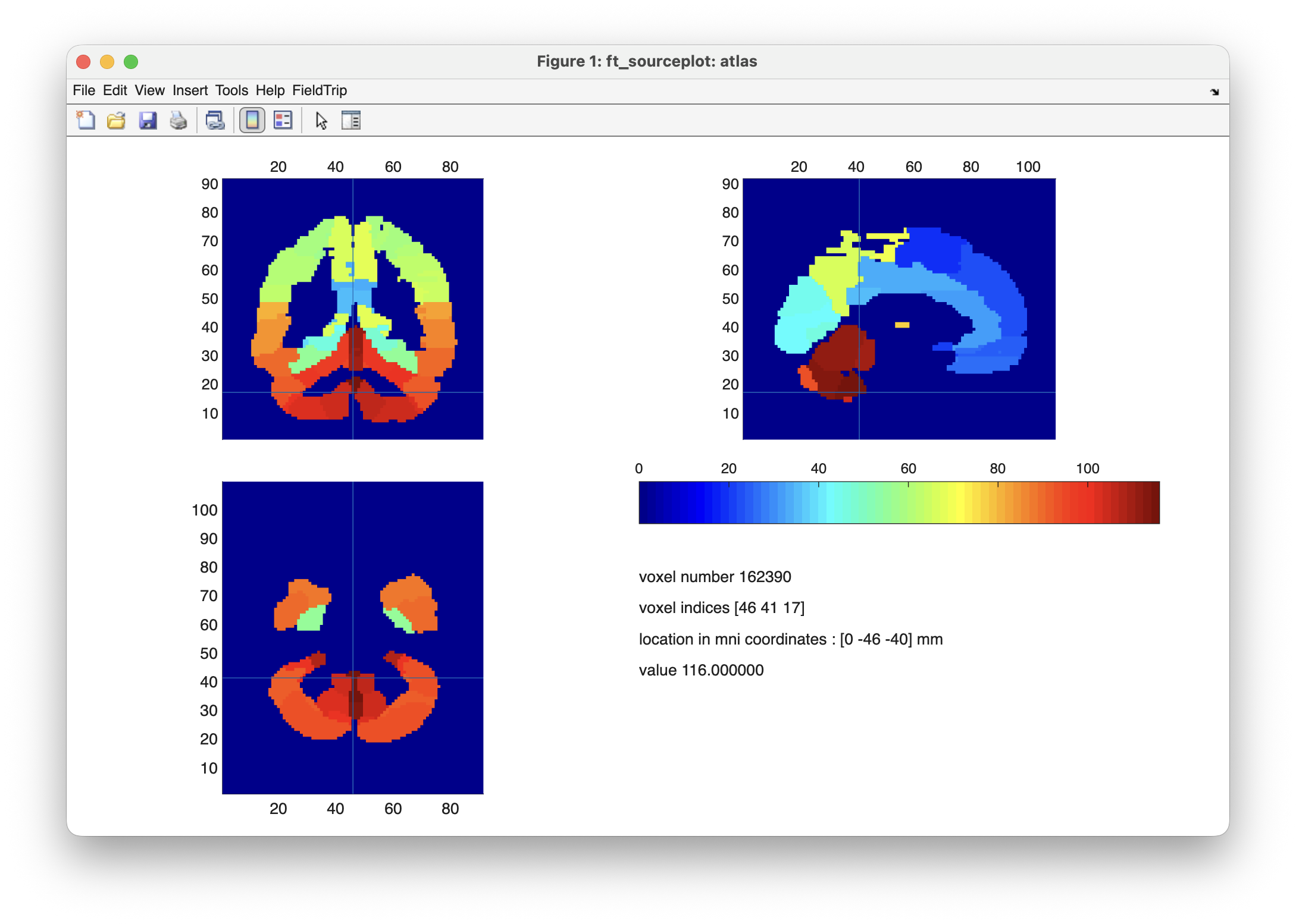
For each vertex of the cortical surface we determine in which atlas voxel it is located. To do that, we apply the inverse of the transformation matrix of the atlas to go from head coordinates to atlas voxel coordinates, and subsequently look up the integer value of the atlas at that voxel.
vox = ft_warp_apply(inv(atlas.transform), cortex.pos);
tissue = zeros(size(cortex.pos,1),1);
for i=1:size(vox,1)
    v = round(vox(i,:));
    if v(1)>=1 && v(1)<=size(atlas.tissue,1) && v(2)>=1 && v(2)<=size(atlas.tissue,2) && v(3)>=1 && v(3)<=size(atlas.tissue,3)
        tissue(i) = atlas.tissue(v(1), v(2), v(3));
    end
end
We can now plot the head surface together with the cortical sheet, colored according to the AAL labels.
figure
ft_plot_headshape(headshape, 'facecolor', 'skin', 'facealpha', 0.2, 'edgecolor', 'none');
ft_plot_mesh(cortex, 'vertexcolor', tissue, 'facealpha', 0.8, 'material', 'dull')
ft_colormap(rand(116,3))
ft_headlight
colorbar
view([-90 0])

Design the OPM helmet
Now that we have the head shape, we can design the helmet. The idea is that the helmet is placed at a fixed distance from the head, leaving a small gap for the hair and some air. Starting from the scalp segmentation, we inflate the scalp with the image processing function imdilate to get an air gap of one voxel (1 mm) and then the helmet shell of 5 mm.
mri_segmented = ft_checkdata(mri_segmented, 'segmentationstyle', 'probabilistic')

mri_segmented.airgap = imdilate(mri_segmented.scalp, strel('sphere', 1));
mri_segmented.helmet = imdilate(mri_segmented.airgap, strel('sphere', 5));
We construct the meshes of the inside and the outside of the helmet.
cfg = [];
cfg.method = 'projectmesh';
cfg.numvertices = 4000;

cfg.tissue = 'airgap';
tmp = removefields(mri_segmented, {'scalp', 'helmet'});
inside = ft_prepare_mesh(cfg, tmp);

cfg.tissue = 'helmet';
tmp = removefields(mri_segmented, {'scalp', 'airgap'});
outside = ft_prepare_mesh(cfg, tmp);
We plot the outside of the helmet together with the head shape.
figure
ft_plot_headshape(headshape, 'facecolor', 'skin', 'facealpha', 0.5, 'edgecolor', 'none');
ft_plot_mesh(outside, 'facecolor', 'lightgray', 'facealpha', 0.5, 'edgecolor', 'none');
ft_headlight
view([90 0])

The helmet mesh extends all the way to the nose and the bottom is closed. In the full OPM helmet design tutorial the face, ears and neck are subsequently cut out of the helmet, and holes for the sensor holders and a chin strap are added, using 3D design software like Fusion or SolidWorks.
Placing OPM sensors according to the 10-20 system
Anatomical landmarks
To position the sensors at the locations of the extended 10-20 system, ft_electrodeplacement needs the position of the anatomical landmarks. For the colin27 template the following approximate positions apply (in mm, MNI coordinates). For an individual MRI you would determine these interactively, e.g. by clicking on the MRI in ft_sourceplot.
headshape.coordsys = 'mni';

nas = [  0.0083   86.8110  -39.9830];
ini = [  0.0045 -118.5650  -23.0780];
lpa = [-86.0761  -19.9897  -47.9860];
rpa = [ 85.7939  -20.0093  -48.0310];

headshape.fid.label = {'nas', 'ini', 'lpa', 'rpa'};
headshape.fid.pos = [nas; ini; lpa; rpa];
Placing the 10-20 electrode positions
We place all positions of the extended 10-20 system on the head shape.
cfg = [];
cfg.fiducial.nas = nas;
cfg.fiducial.ini = ini;
cfg.fiducial.lpa = lpa;
cfg.fiducial.rpa = rpa;
cfg.method = '1020'; % this results in the 5% system, see Oostenveld et al 2001
cfg.feedback = 'yes';
elec = ft_electrodeplacement(cfg, headshape);
This results in more than 300 electrode positions on the head shape, not only including the 20% positions but also the 10% and the 5% positions. We take the standard 10-20 montage with 19 positions, excluding Fpz and Oz. The actual number of sensors depends on the OPM system you have, here we use a small set to keep it simple.
chansel = ft_channelselection({'eeg1020', '-Fpz', '-Oz'}, elec.label);
We plot the 19 electrode positions on the head surface.
cfg = [];
cfg.channel = chansel;
elec19 = ft_electrodeselection(cfg, elec);

figure
ft_plot_headshape(headshape, 'facecolor', 'skin', 'facealpha', 0.5, 'edgecolor', 'none');
ft_plot_sens(elec19, 'label', 'label', 'fontsize', 8);
ft_headlight
view([90 0])

Placing the OPM sensors on the helmet
We use ft_sensorplacement to rotate and translate the 3D model of the sensor to each of the 19 selected positions. The function shifts the object with cfg.outwardshift in the direction perpendicular to the surface, and subsequently translates it to the final position. The bottom of the sensor holder is placed halfway in the 5 mm thick helmet wall, which is 1 mm above the scalp, hence the cfg.outwardshift of 1 + 5/2 mm.
cfg = [];
cfg.elec = elec;
cfg.channel = chansel;
cfg.outwardshift = 1 + 5/2;

cfg.template = 'fieldline_sensor.stl';
[outcfg, sensor] = ft_sensorplacement(cfg, headshape);

cfg.template = 'fieldline_holder.stl';
[outcfg, holder] = ft_sensorplacement(cfg, headshape);

cfg.template = 'fieldline_padding.stl';
[outcfg, padding] = ft_sensorplacement(cfg, headshape);

cfg.template = 'fieldline_hole.stl';
[outcfg, hole] = ft_sensorplacement(cfg, headshape);
We plot the sensors on the helmet. We could also plot the OPM sensor holders and/or the holes that need to be made in the 3D printed helmet to glue the holders in.
figure
ft_plot_headshape(headshape, 'facecolor', 'skin', 'facealpha', 0.5, 'edgecolor', 'none');
ft_plot_mesh(outside, 'facecolor', 'lightgray', 'facealpha', 0.3, 'edgecolor', 'none');
ft_plot_mesh(sensor, 'facecolor', 'r', 'facealpha', 1, 'edgecolor', 'none');
% ft_plot_mesh(holder, 'facecolor', 'g', 'facealpha', 1, 'edgecolor', 'none');
ft_headlight
view([90 0])

Constructing the gradiometer definition
For the analysis we need a grad_xyz structure that specifies for each channel the position, orientation and label. We assume that each OPM sensor measures the magnetic field in three orthogonal directions, which we will call x, y and z. We define a single OPM sensor with three channels as a template.
opm_single = [];
opm_single.label = {
    'x'
    'y'
    'z'
};
opm_single.coilpos = [
    0 0 0
    0 0 0
    0 0 0
];
opm_single.coilori = [
    1 0 0
    0 1 0
    0 0 1
];
opm_single.tra = eye(3);
We again use ft_sensorplacement, but now with this sensor template rather than with the STL model. The cfg.outwardshift needs to be 1 + 5/2 + 1 + 5 mm: the air gap is 1 mm, the bottom of the sensor holder is halfway in the 5 mm thick helmet wall, the bottom of the sensor is located 1 mm above the bottom of the holder, and the OPM sensor measures the field at a spot 5 mm from its bottom.
cfg = [];
cfg.elec = elec;
cfg.channel = chansel;
cfg.template = opm_single;
cfg.outwardshift = 1 + 5/2 + 1 + 5;
[outcfg, opm_all] = ft_sensorplacement(cfg, headshape);
The output opm_all is a structure array with one element for each of the 19 sensors, where each sensor represents three channels. We combine all channels into a single grad_xyz structure.
grad_xyz = [];
grad_xyz.label = {};
grad_xyz.coilpos = zeros(0,3);
grad_xyz.coilori = zeros(0,3);
for i=1:length(chansel)
    lab{1} = [outcfg.channel{i} '_' opm_all(i).label{1}]; % _x
    lab{2} = [outcfg.channel{i} '_' opm_all(i).label{2}]; % _y
    lab{3} = [outcfg.channel{i} '_' opm_all(i).label{3}]; % _z
    grad_xyz.label = cat(1, grad_xyz.label, lab(:));
    grad_xyz.coilpos = cat(1, grad_xyz.coilpos, opm_all(i).coilpos);
    grad_xyz.coilori = cat(1, grad_xyz.coilori, opm_all(i).coilori);
end
grad_xyz.tra = eye(length(grad_xyz.label));
We plot the resulting grad_xyz structure with all 57 channels (19 sensors times 3 orientations).
figure
ft_plot_headshape(headshape, 'facecolor', 'skin', 'facealpha', 0.5, 'edgecolor', 'none');
ft_plot_sens(grad_xyz);
ft_headlight
view([90 0])

For the topographic maps and the sensitivity it is often easier to look at only the radially oriented channels, i.e. the channels in the z-direction of the sensor.
figure
ft_plot_headshape(headshape, 'facecolor', 'skin', 'facealpha', 0.5, 'edgecolor', 'none');
ft_plot_sens(grad_xyz, 'chanindx', endsWith(grad_xyz.label, 'z'), 'label', 'label', 'fontsize', 8);
ft_headlight
view([90 0])

Selecting a subset of OPM sensors
In this tutorial we are assuming that we have an OPM system with only a limited number of OPM sensors that we want to place optimally for a specific research question, for example over a specific brain region. The selection of channels is done with ft_electrodeselection, which works both on the channel labels and on the channel indices.
First we select the radially oriented channels. In the grad_xyz structure each OPM sensor contributes an x, a y and a z channel at the same position, and the channels that we will use for the sensitivity analysis are the radially oriented ones, i.e. those with the _z suffix.
cfg = [];
cfg.channel = endsWith(grad_xyz.label, '_z');
grad_z = ft_electrodeselection(cfg, grad_xyz);
As an example of a research question, let us assume that we are interested in the sensorimotor cortex, and hence want to cover the central and parietal cortex with a small number of sensors. We select the channels at C3, Cz, C4, P3, Pz and P4.
cfg = [];
cfg.channel = {'C3_z', 'Cz_z', 'C4_z', 'P3_z', 'Pz_z', 'P4_z'};
grad_sel = ft_electrodeselection(cfg, grad_z);
For the FieldLine v3 OPM sensors it is recommended to only work with the two orientations by and bz, since the sensitivity of the bx channel is along the direction of the laser and is very noisy. In the design above we only work with the _z channels, which correspond to the radial bz orientation.
If you have a FieldLine Beta2 smart helmet, the positions of all 144 slots in the helmet are available as a template gradiometer definition, and you can select the slots in which to place your OPM sensors in exactly the same way, for example every 4th slot.
[ftver, ftpath] = ft_version;
fieldlinebeta2 = ft_read_sens(fullfile(ftpath, 'template/gradiometer/fieldlinebeta2.mat'));
fieldlinebeta2 = ft_convert_units(fieldlinebeta2, 'm');

cfg = [];
cfg.channel = 1:4:144; % select every 4th slot, this gives 144/4=32 sensors
fieldlinebeta2_sel = ft_electrodeselection(cfg, fieldlinebeta2);
For the interactive selection of sensor positions, e.g. by clicking on a 3D rendering of the helmet with all sensors, you can also use ft_electrodeselection with the 3D model of the sensors as input. See the example on selecting a subset of OPM sensor positions for details.
Plotting the sensitivity map
To see how well the selected sensor positions cover the brain, we compute the sensitivity map, i.e. for every vertex on the cortical surface how sensitive the sensor array is to a source at that location. For that we need a volume conduction model of the head, a source model, and the lead fields.
Volume conduction model
We use the template head model that is included with FieldTrip, and compute a single-shell volume conduction model of the brain.
[ftver, ftpath] = ft_version;
mri_seg = ft_read_mri(fullfile(ftpath, 'template/headmodel/standard_seg.mat'));
mri_seg.coordsys = 'mni';
mri_seg.seglabel = {'scalp', 'skull', 'brain'};

cfg = [];
cfg.tissue = 'brain';
cfg.method = 'singleshell';
headmodel = ft_prepare_headmodel(cfg, mri_seg);
Source model
We use the same template cortical sheet as before as the source model.
[ftver, ftpath] = ft_version;
sourcemodel = ft_read_headshape(fullfile(ftpath, 'template/sourcemodel/cortex_20484.surf.gii'));
Leadfields
We compute the leadfields for the full array and for the subset of 6 sensors, using the same source model. The forward model computation is done in SI units, so we convert the head model, source model and sensor positions to m. The cfg.orientation = 'yes' ensures that the cortical surface normal is included in the source model, which we need for the fixed-orientation sensitivity.
cfg = [];
cfg.headmodel = ft_convert_units(headmodel, 'm');
cfg.sourcemodel = ft_convert_units(sourcemodel, 'm');
cfg.sourcemodel.inside = ones(size(sourcemodel.pos,1), 1);
cfg.orientation = 'yes';

cfg.grad = ft_convert_units(grad_z, 'm');
lf_z = ft_prepare_leadfield(cfg);

cfg.grad = ft_convert_units(grad_sel, 'm');
lf_sub = ft_prepare_leadfield(cfg);
Compute the sensitivity
We compute the sensitivity for every source position with a helper function that is copied from the sensitivity maps tutorial. The free sensitivity is the largest singular value of the lead field matrix, and is a measure for how sensitive the array is for a source with free orientation. The fixed sensitivity projects the lead field onto the known cortical surface normal, and the distance is the distance from the source to the nearest channel. Copy the following code and save it as ft_sensitivitymap.m in your current directory.
function sourcemodel = ft_sensitivitymap(cfg, sourcemodel)

% FT_SENSITIVITYMAP computes various measures of sensitivity

sourcemodel.free     = nan(size(sourcemodel.pos,1), 1);
sourcemodel.fixed    = nan(size(sourcemodel.pos,1), 1);
sourcemodel.distance = nan(size(sourcemodel.pos,1), 1);

% ensure that it has chanpos
cfg.grad = ft_datatype_sens(cfg.grad);

for i=1:size(sourcemodel.pos,1)
    [u, s, v] = svd(sourcemodel.leadfield{i}, 'econ');
    sourcemodel.free(i) = s(1);

    [u, s, v] = svd(sourcemodel.leadfield{i} * (sourcemodel.ori(i,:)'), 'econ');
    sourcemodel.fixed(i) = s(1);

    % compute the distance of all channels to this source
    d = cfg.grad.chanpos;
    d(:,1) = d(:,1) - sourcemodel.pos(i,1);
    d(:,2) = d(:,2) - sourcemodel.pos(i,2);
    d(:,3) = d(:,3) - sourcemodel.pos(i,3);
    d = sqrt(sum(d.^2, 2));

    sourcemodel.distance(i) = min(d); % take the smallest distance
end

% only keep the relevant fields
sourcemodel = keepfields(sourcemodel, {'pos', 'tri', 'ori', 'unit', 'free', 'fixed', 'distance'});
We now compute the sensitivity for both arrays.
cfg = [];
cfg.grad = ft_convert_units(grad_z, 'm');
sens_z = ft_sensitivitymap(cfg, lf_z);

cfg = [];
cfg.grad = ft_convert_units(grad_sel, 'm');
sens_sub = ft_sensitivitymap(cfg, lf_sub);
Plot the sensitivity maps
We plot the relative sensitivity (the sensitivity scaled to the most sensitive source) for the full array with all 19 sensors.
maxval = max(sens_z.free);

figure
ft_plot_mesh(sourcemodel, 'vertexcolor', sens_z.free ./ maxval)
ft_plot_sens(ft_convert_units(grad_z, 'mm'), 'label', 'label', 'fontsize', 8)
ft_colormap('jet')
clim([0 1])
colorbar
title('relative sensitivity, full array')
view([-90 0])

and for the subset with only 6 sensors over the sensorimotor cortex.
figure
ft_plot_mesh(sourcemodel, 'vertexcolor', sens_sub.free ./ maxval)
ft_plot_sens(ft_convert_units(grad_sel, 'mm'), 'label', 'label', 'fontsize', 8)
ft_colormap('jet')
clim([0 1])
colorbar
title('relative sensitivity, subset')
view([-90 0])

You can see that the full array covers the whole brain, whereas the subset of 6 sensors is only sensitive to the source locations in the sensorimotor cortex, which is what we aimed for. So a small OPM system with 6 channels can quite well record activity from a limited brain region, whereas an OPM system with 57 channels (or more) is able to record from the whole brain.
Exercise
Consider the sensitivity difference of the whole-head OPM system for superficial and for deep sources. Is that what you expected?
The advantage of a small but well-placed sensor array like the one with 6 radial OPM channels is that we can quite well record activity from the region of interest, but the lack of sensitivity to other brain regions means that we cannot tell anything about the presence or absence of activity elsewhere.
Summary and suggested further reading
In this tutorial we planned the acquisition of OPM-MEG data. We read and segmented the colin27 template MRI, made a mesh of the head surface, and visualized it together with the template cortical sheet and the AAL anatomical labels. We designed an OPM helmet by inflating the scalp segmentation, placed OPM sensors at the 19 positions of the standard 10-20 system, and constructed the grad_xyz structure that specifies the position and orientation of all 57 channels (19 sensors times 3 orientations). Finally, we selected a subset of 6 channels over the sensorimotor cortex and plotted the sensitivity map for both the full array and the subset, which showed how the selection of sensor positions determines the brain regions that the sensor array is sensitive to.
See also
For more information, see also the following tutorials:
- Coregistration of Optically Pumped Magnetometer (OPM) data
- Denoising OPM data
- Designing a custom 3D printed OPM helmet
- Using a MEG phantom for validation and OPM calibration
- Preprocessing of Optically Pumped Magnetometer (OPM) data
- Comparing MEG sensitivity maps for SQUID and OPM sensor arrays
and the following examples: