documentation / tutorial / preproc / denoising_opm /
Denoising OPM data
Introduction
Optically pumped magnetometers (OPMs) offer flexible and wearable MEG recordings, but are particularly susceptible to environmental noise and movement artifacts. This tutorial demonstrates how to apply various denoising techniques to OPM data using FieldTrip, with a focus on visual evoked field (VEF) recordings.
An important difference between OPM-based and SQUID-based MEG systems is that OPMs are magnetometers, whereas most conventional MEG systems consist of (mostly) gradiometers. Gradiometers are designed to suppress the environmental field, as explained in this video. Magnetometers see more of the environmental noise and consequently the static earth magnetic field can also become visible as noise due to (small) movements. Movements of the head, and thereby of the sensors, cause the OPMs to move through the residual earth magnetic field in the magnetically shielded room (MSR). As head movements are relatively slow, this results in low-frequency noise. In addition, vibrations of the MSR may also add higher frequency components to the noise. Finally, other sources of artifacts, e.g. due to electrical equipment, may also be readily picked up by the sensors.
This tutorial focusses on the (software-based) denoising of OPM data and evaluates the effect of various types of denoising on the outcome of simple ERF analyses. Following the denoising, you could you could in principle continue with any regular type of sensor- or source-level analysis. For instance, computation of the event-related fields, or event-related (de)synchronization by means of a time-frequency analysis, could be followed by dipole fitting, or beamformer source reconstruction.
In this tutorial you will learn:
- How to characterize and analyze emptyroom noise data
- How to apply signal space projection (SSP) for noise suppression
- How to use harmonic field correction (HFC) for environmental noise removal
- How to apply adaptive multipole modeling (AMM) for motion artifact cleaning
- How to compare the effectiveness of different denoising approaches
This tutorial assumes that you have some experience with MEG data and are familiar with the basic preprocessing workflow. It focuses specifically on denoising techniques for OPM data. For a more general introduction to MEG preprocessing see the event-related averaging and MEG planar gradient tutorial and for OPM data processing see the OPM preprocessing tutorial.
The denoising techniques demonstrated here are particularly relevant for OPM recordings in environments with residual magnetic fields, where movement artifacts and environmental noise can significantly degrade data quality. Note that denoising is not a substitute for good experimental design - proper MSR shielding, nulling coils, and minimizing participant movement are still essential.
Background
OPM sensors are extremely sensitive to magnetic fields, which makes them susceptible to various sources of noise:
- Environmental noise: Residual magnetic fields in the MSR and external magnetic sources
- Movement artifacts: OPMs moving through the residual magnetic field generate large artifacts
- Biological artifacts: Cardiac and muscle activity that is not of interest
All denoising techniques that we are going to explore in this tutorial are so-called spatial filtering techniques, which regress out a spatio(-temporal) model of the ambient magnetic field from the data. This model of the ambient magnetic field is obtained from signals of the same sensors as the ones that we want to denoise. As such this strategy has been used in SQUID-MEG analysis as well, specifically in data from Elekta/Neuromag systems. Practically, each sensor’s MEG signal will be replaced by a weighted combination of all channels’ data. The different flavours of denoising algorithms differ in the way that the spatial weights are computed.
Signal space projection (SSP) is an established technique that uses a principal component analysis (PCA) based spatial decomposition of (typically) emptyroom data to remove components that have large variance. Using emptyroom data avoids actual brain signals to contaminate the noise model estimation process, but requires the sensors to be in a position - both within the MSR and in relation to one another - that is as similar as possible as during the actual recording(s) of interest. For SQUID-MEG this means that different SSP filters are needed for upright and supine measurements. For OPMs this be difficult to achieve in practice, even with a fixed helmet mount, when individual sensors are slightly moved inward in order to touch the scalp surface, or to move outward in order for the participant to move into and out of the helmet. Thus, alternatively, one may consider to use (parts of) the actual recording-of-interest for the estimation of the spatial projectors. Although these data will invariably contain relevant brain-related activity, if the ambient noise is a few orders of magnitude stronger than the brain signals, the signal space projectors may still sufficiently well capture the noise. In FieldTrip this algorithm is implemented in ft_denoise_ssp.
Harmonic field correction (HFC) creates a model of the low spatial frequency components of the magnetic field distribution. This approach requires geometric information, the relative sensor positions, and is based on the underlying assumption that the low spatial frequency components originate from (ambient) sources that are located far away from the sensors. In FieldTrip this algorithm is implemented in ft_denoise_hfc.
Signal Space Separation (SSS) is an established technique for cleaning Megin/Elekta/Neuromag data and also known as MaxFilter, but can theoretically be applied to other sensor configurations as well. The approach creates a spatial model, separating signal contributions originating from inside and outside the sensor-helmet, followed by an optional temporal regression step for further cleaning. It requires geometric information of the sensors. In FieldTrip this algorithm is implemented in ft_denoise_sss.
Adaptive multipole modeling (AMM) is a variant of SSS, using slightly different heuristics, such as the basis functions for the model. It requires geometric information of the sensors. In FieldTrip this algorithm is implemented in ft_denoise_amm.
Dual signal subspace projection (DSSP) uses - just like SSS and AMM - a combination of a spatial model and temporal regression for cleaning. It requires geometric information of the sensors and a volume conduction model and brain source model for biophysical forward modeling. In FieldTrip this algorithm is implemented in ft_denoise_dssp.
Here, we will explore the effect of some of those strategies.
The dataset used in this tutorial
OPM recordings were done using a FieldLine v3 system comprised of between 131 and 133 OPMs sensitive in the radial (or axial) direction. The OPMs were placed in a FieldLine beta-2 smart helmet, which allows them to be slided inwards, touching the scalp surface. Moreover, using the smart helmet allows for automatic coregistration of the OPM sensors (relative to the helmet), resulting in data with accurate position information of the individual sensors. The data used here have been further processed to be coregistered to the participant’s head based coordinate system. To this end, a separate recording had been performed, during which the HPI-coils attached to the participant were localized. Subsequently the channel position information in the recordings (expressed in smart helmet coordinates) were replaced with the channel positions in head coordinates. Here we will explore the emptyroom recording, and a recording during which visual stimuli were presented in the left upper visual quadrant.
The data for this tutorial can be downloaded here from our download server. You need to download the zip-file, and unpack it.
Procedure
The tutorial follows these steps:
- Load and analyze emptyroom data to characterize the noise environment, using ft_preprocessing, ft_freqanalysis, ft_componentanalysis, and ft_icabrowser.
- Preprocess and explore the task data, using ft_preprocessing, ft_timelockanalysis, ft_multiplotER.
- Apply SSP denoising using emptyroom data and task data for comparison, using ft_denoise_ssp, visualizing the results with ft_topoplotER
- Apply HFC denoising for environmental noise removal, using ft_denoise_hfc
- Apply AMM denoising for movement artifact correction, using ft_denoise_amm
Analyzing the emptyroom recording
We start by loading the emptyroom data. This allows us to characterize the noise environment and identify potential noise components that can be removed from the task data.
datadir = '<PATH-TO>/tutorialdata/sub-001/ses-opm01/meg'; % NOTE this needs to be changed to match your computer
dataset = fullfile(datadir, 'sub-001_ses-opm01_task-emptyroom_meg.fif');

% first pass for exploration, to evaluate the power spectrum, and perform PCA
cfg         = [];
cfg.dataset = dataset;
data_er     = ft_preprocessing(cfg);
The emptyroom data is loaded using ft_preprocessing with default settings. This gives us a first look at the raw data structure.
Next, we perform frequency analysis to examine the spectral characteristics of the noise:
cfg = [];
cfg.method = 'mtmfft';
cfg.taper  = 'hanning';
cfg.channel = 'MEG';
freq_er = ft_freqanalysis(cfg, data_er);

cfg = [];
cfg.operation = 'log10';
cfg.parameter = 'powspctrm';
freq_er = ft_math(cfg, freq_er);

figure
subplot(121); plot(freq_er.freq, freq_er.powspctrm); xlim([0 80]);
subplot(122); plot(freq_er.freq, freq_er.powspctrm); xlim([0 500]);
Here we use ft_freqanalysis with multitaper frequency estimation and Hanning taper to compute the power spectrum. The ft_math function applies a log10 transformation to make the spectral peaks more visible. The two subplots show the spectrum in different frequency ranges: 0-80 Hz (left) for the lower frequency range, mostly relevant for our neural signal analysis, and the full 0-500 Hz (right).
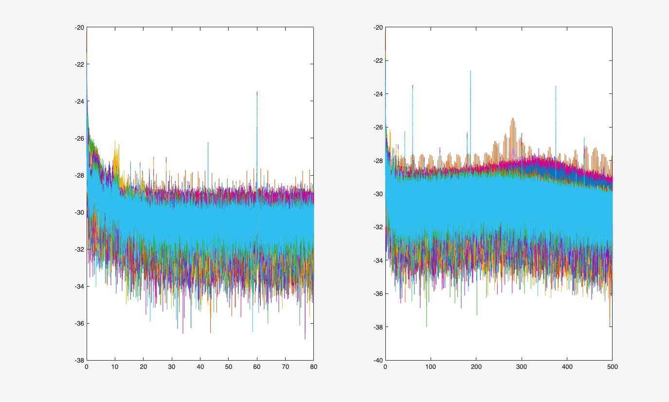
The power spectrum of the emptyroom data helps identify characteristic noise peaks. In a well-shielded MSR, you might see peaks at line noise frequencies (50 or 60 Hz and harmonics), but residual environmental noise may still be present, especially at lower frequencies.
To reduce the variance in the spectrum, we can cut the data into shorter segments, compute the spectrum per segment, and then average across segments. This is very similar to Welch’s periodogram method:
cfg         = [];
cfg.length  = 2;
data_er     = ft_redefinetrial(cfg, data_er);

cfg = [];
cfg.method = 'mtmfft';
cfg.taper  = 'hanning';
cfg.channel = 'MEG';
freq_er = ft_freqanalysis(cfg, data_er);

cfg = [];
cfg.operation = 'log10';
cfg.parameter = 'powspctrm';
freq_er = ft_math(cfg, freq_er);

figure
subplot(121); plot(freq_er.freq, freq_er.powspctrm); xlim([0 80]);
subplot(122); plot(freq_er.freq, freq_er.powspctrm); xlim([0 500]);
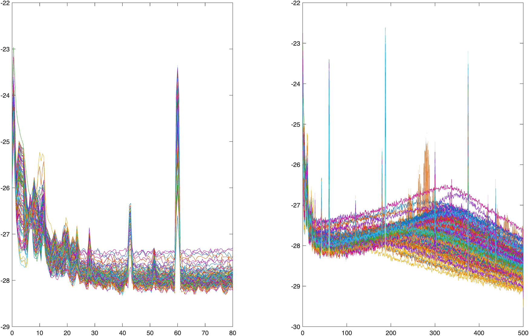
The ft_redefinetrial function cuts the continuous data into 2-second segments, which helps reduce the memory requirements and improves the spectral estimation.
We can visualize the spatial distribution of noise across sensors using a butterfly plot:
cfg        = [];
cfg.layout = 'fieldlinebeta2bz_helmet.mat';
cfg.linecolor = 'spatial';
cfg.viewmode  = 'butterfly';
ft_multiplotER(cfg, freq_er);
The ft_multiplotER function with ‘butterfly’ viewmode shows all sensor traces overlaid, with the ‘spatial’ linecolor option coloring each sensor differently. This helps identify sensors with unusual noise patterns.
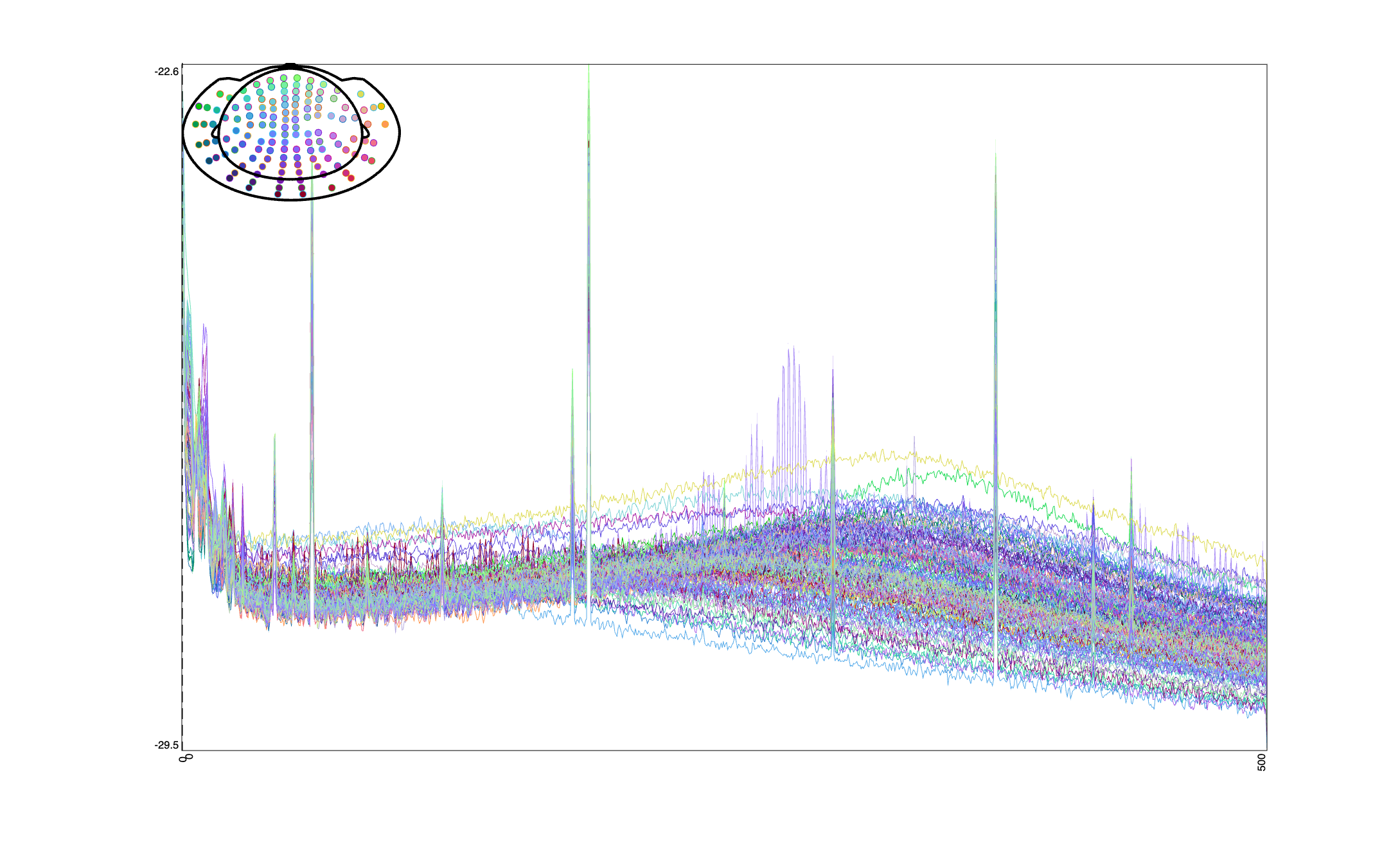
Exploring the topographies of low-frequency power often reveals spatially structured ambient noise patterns. These smooth topographies are candidate components for SSP-based noise suppression. The figure that you have just created is interactive, so you can left-click and drag to select a certain frequency range that can be displayed topographically.
Exercise
Explore the spectra by selecting several frequency ranges and evaluate the topographical distribution.
To identify spatial noise components, we can also perform principal component analysis (PCA):
cfg = [];
cfg.method = 'pca';
cfg.channel = 'MEG';
comp_er = ft_componentanalysis(cfg, data_er);

cfg        = [];
cfg.layout = 'fieldlinebeta2bz_helmet.mat';
[rej, art] = ft_icabrowser(cfg, comp_er);
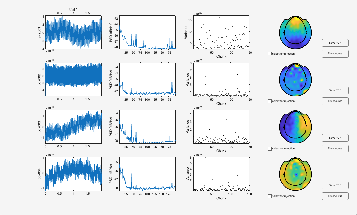
The ft_componentanalysis function performs PCA on the emptyroom data. The ft_icabrowser function provides an interactive interface to visualize the components and identify noise-related topographies. This function is not in the ‘core’ FieldTrip folder, but has been contributed by external contributors.
Exercise
Examine the PCA components in the icabrowser interface. Which components show smooth spatial patterns that are characteristic of ambient noise? Which components show more focal patterns that might represent sensor-specific noise?
Note: Some of the PCs may show smooth patterns, but they are not necessarily the first ordered PCs. For example, component 2 might be not a good candidate for SSP. This indicates that the quality of the (emptyroom) recording may be insufficient to automatically capture the main noise components in the first few PCs. This is relevant for the algorithmic implementation of the SSP-algorithm below, which will by default remove the first ‘N’ spatial components from the data.
The previous analysis showed that the raw emptyroom data might be too noisy to reliably identify the main noise components in the first ‘N’ PCs. Part of this may be caused by high variance noise characteristics, e.g. powerline related artifacts may be sensor specific. We can improve this by applying appropriate time-domain filters:
cfg = [];
cfg.dataset = dataset;
cfg.bpfilter = 'yes';
cfg.bpfreq   = [1 80];
cfg.bpfilttype = 'firws';
cfg.bsfilter  = 'yes';
cfg.bsfreq    = [58 62];
cfg.bsfilttype = 'firws';
data_er = ft_preprocessing(cfg);

cfg         = [];
cfg.length  = 2;
data_er     = ft_redefinetrial(cfg, data_er);

cfg = [];
cfg.method = 'pca';
cfg.channel = 'MEG';
comp_er = ft_componentanalysis(cfg, data_er);

cfg        = [];
cfg.layout = 'fieldlinebeta2bz_helmet.mat';
[rej, art] = ft_icabrowser(cfg, comp_er);
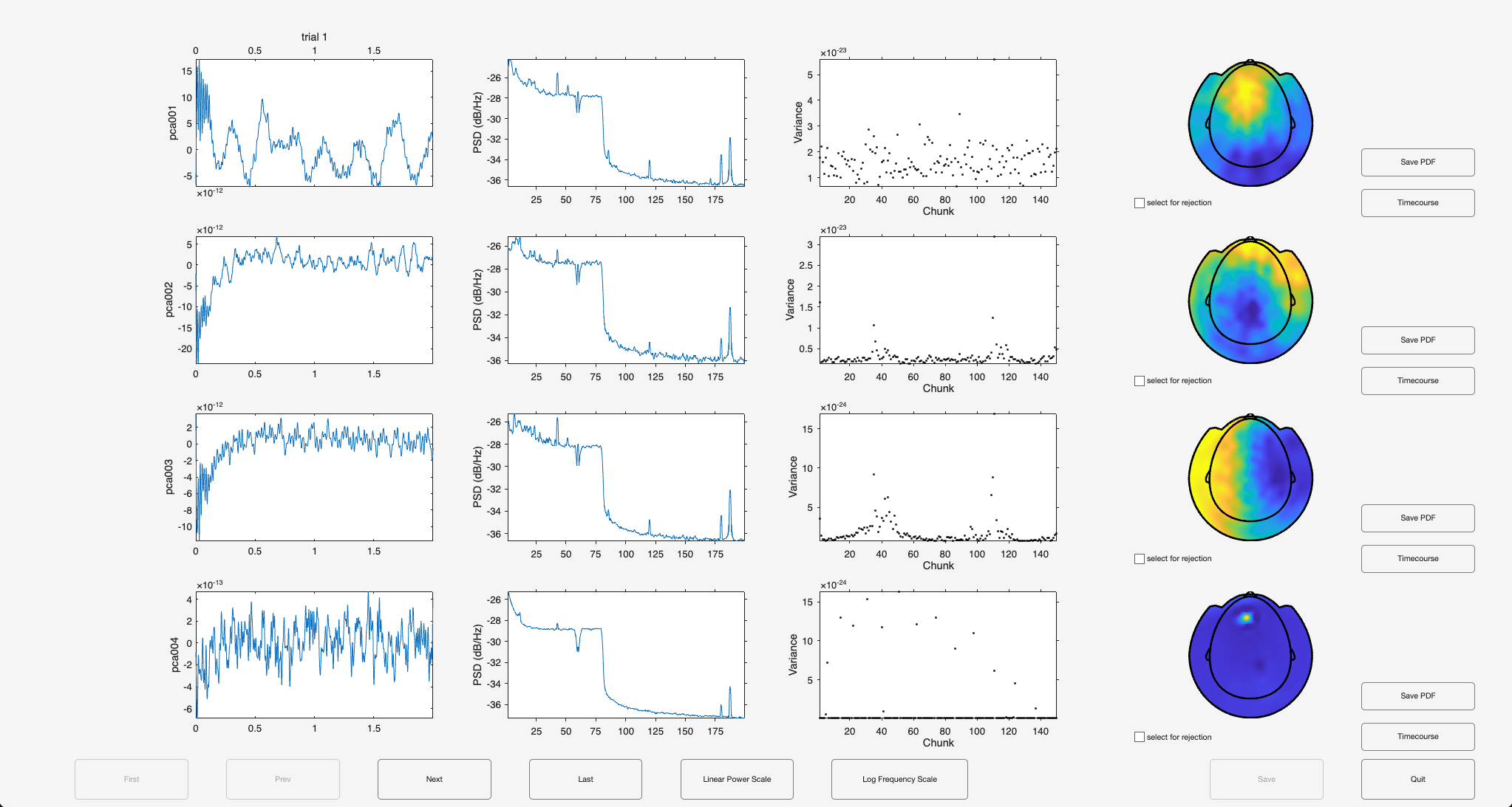
Here we applied a bandpass filter (1-80 Hz) and a bandstop filter (58-62 Hz) to remove line noise using ft_preprocessing.
Exercise
Examine the topographies and time courses of the PCs, and compare them to the PCs obtained from the unfiltered data. What has changed? How many components would you identify as candidates for the SSP?
Loading and preprocessing the task data
Now we load the visual evoked field (VEF) task data:
dataset = fullfile(datadir, 'sub-001_ses-opm01_task-veful_meg.fif');

cfg                    = [];
cfg.dataset            = dataset;
cfg.trialdef.eventtype = 'stim_onset';
cfg.trialdef.prestim   = 0.1;
cfg.trialdef.poststim  = 0.5;
cfg = ft_definetrial(cfg);

cfg.bpfilter = 'yes';
cfg.bpfilttype = 'firws';
cfg.bpfreq = [1 80];
cfg.demean = 'yes';
cfg.padding = 4;
cfg.baselinewindow = [-0.1 0];
cfg.bsfilter = 'yes';
cfg.bsfreq  = [58 62];
cfg.bsfilttype = 'firws';
cfg.channel = data_er.label;
data = ft_preprocessing(cfg);
We use ft_definetrial to segment the continuous data into trials based on ‘stim_onset’ events, with 0.1 seconds pre-stimulus and 0.5 seconds post-stimulus. The preprocessing includes the same bandpass and bandstop filters as before, plus baseline correction.
Next, we compute the event-related fields (ERFs) by averaging across trials:
cfg = [];
cfg.channel = 'MEG';
tlck = ft_timelockanalysis(cfg, data);

cfg        = [];
cfg.layout = 'fieldlinebeta2bz_helmet.mat';
cfg.linecolor = 'spatial';
cfg.viewmode = 'butterfly';
ft_multiplotER(cfg, tlck);
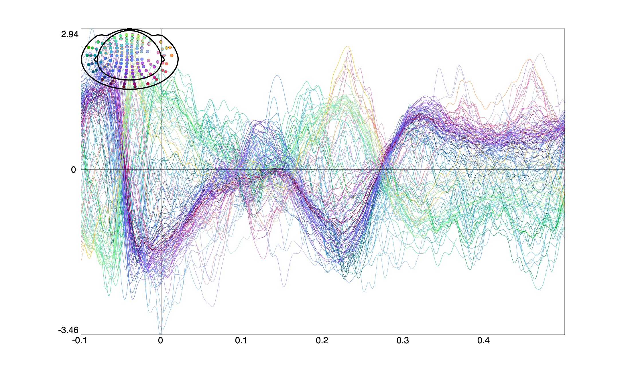
The ft_timelockanalysis function computes the average ERF across trials, and we visualize it with ft_multiplotER in butterfly mode.
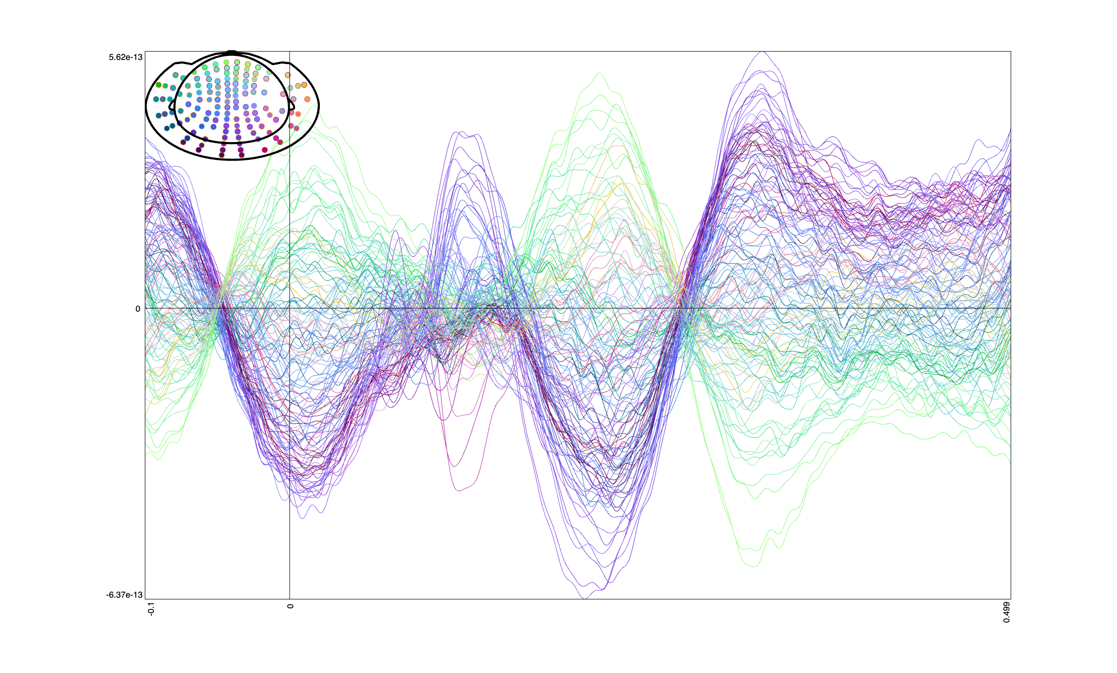
The most striking feature of the above image is antiphasic waxing and waning pattern of the sets of green (frontal) and purple (occipital) sensors. If we select an early latency time window (by left clicking and dragging on top of the open figure) around the first green peak (i.e. around time point 0), we obtain a topography that looks like this:
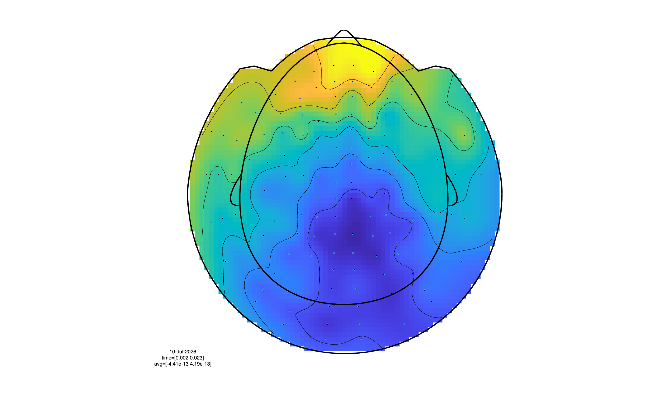
Clearly, this looks very much like the topography of one of the principal components identified in the emptyroom data. Also if we now zoom in on the latency between 70 and 75 ms, we obtain a topography that looks like this:
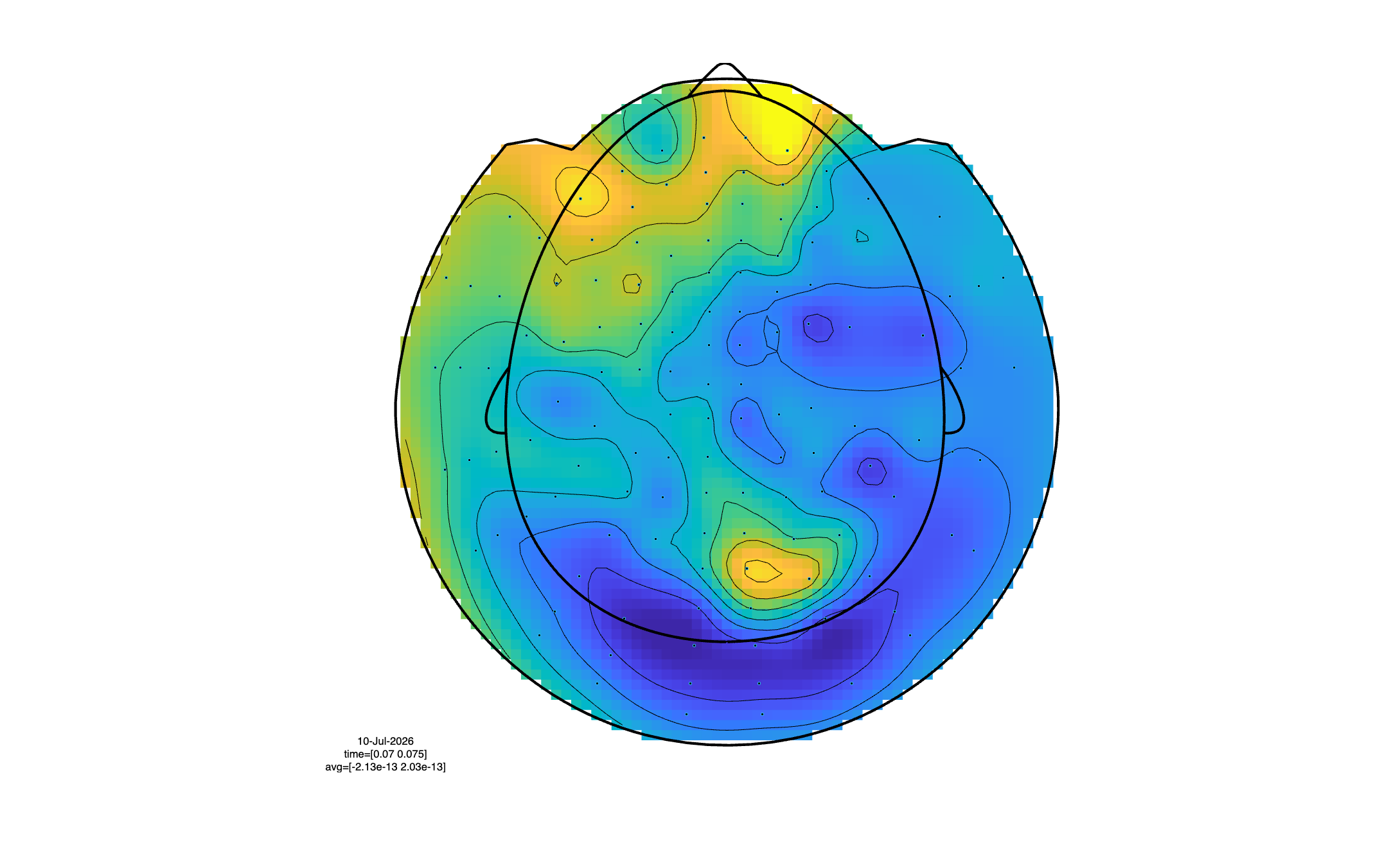
Here, we may observe - albeit faintly - a dipolar visual evoked field pattern with right hemispheric dominance.
Another way of evaluating the quality of the ERF, is to express the single trial data at each time point as a T-statistic against 0. One way to do this would be to use ft_timelockstatistics using single trial data in the input.
cfg            = [];
cfg.channel    = 'MEG';
cfg.keeptrials = 'yes';
tlck_trials    = ft_timelockanalysis(cfg, data);

tlck_trials0 = tlck_trials;
tlck_trials0.trial(:) = 0;

nrpt   = numel(data.trial);
design = [ones(1,nrpt) ones(1,nrpt)*2; 1:nrpt 1:nrpt];

cfg           = [];
cfg.method    = 'analytic';
cfg.statistic = 'depsamplesT';
cfg.design    = design;
stat = ft_timelockstatistics(cfg, tlck_trials, tlck_trials0);

cfg        = [];
cfg.layout = 'fieldlinebeta2bz_helmet.mat';
cfg.linecolor = 'spatial';
cfg.viewmode = 'butterfly';
cfg.parameter = 'stat';
ft_multiplotER(cfg, stat);
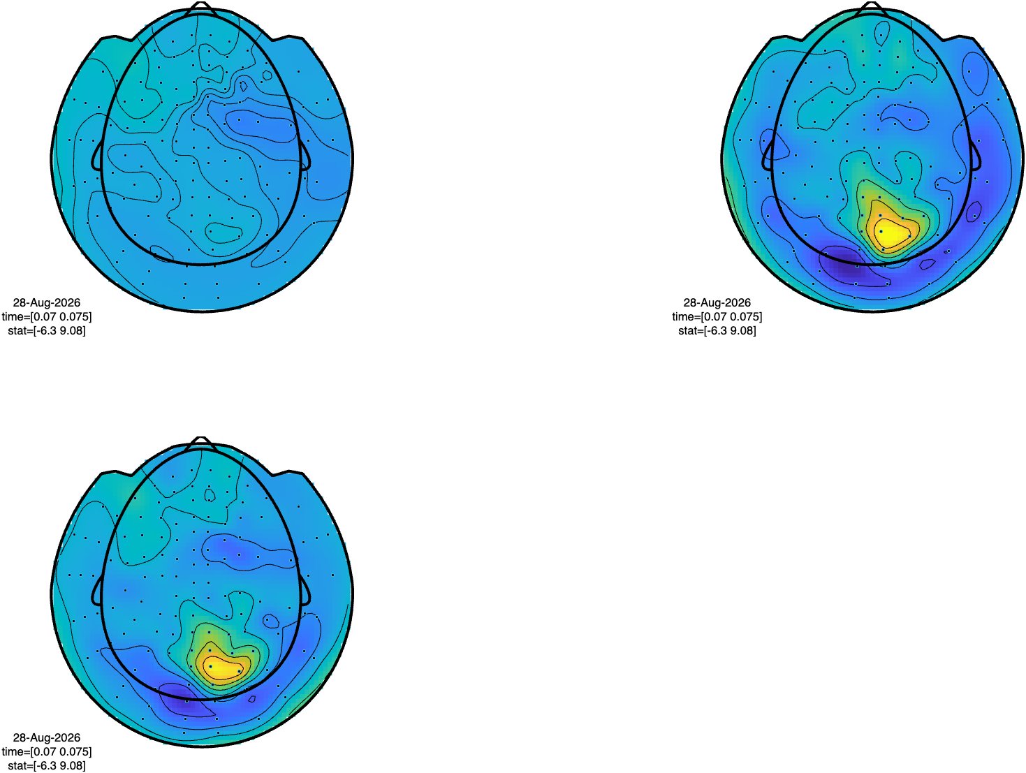
In the above, we have created two data structures, one containing the single trial data in a 3-dimensional #trial x #channel x #time point matrix, and the other one containing a matrix with all zeros. This is needed, because the low-level FieldTrip functions that compute test statistics expect data from 2 conditions in the input. Using a data object with all zeros allows us to compute a T-statistic ‘against 0’. Note that the T-statistic has not been computed here to assess statistical significance, it’s used as a metric to quantify the reliability with which the averaged signals deviate from 0.
Denoising with SSP
Signal Space Projection (SSP) is a technique that removes noise components by projecting the data onto a subspace orthogonal to the noise components. Often these noise components are modeled as the largest principal components, i.e. spatial components that explain most of the variance in the data. We demonstrate two approaches: using the task data itself for SSP estimation, and using the emptyroom data. In the previous section we have seen that even after averaging across multiple trials, the ERF still shows large amplitude fluctuations with a spatial topography that is similar to what we observed in the emptyroom measurement.
% compute the SSPs on-the-fly and clean the task data
cfg = [];
cfg.channel    = 'MEG';
cfg.refchannel = 'MEG';
data_ssp1 = ft_denoise_ssp(cfg, data, data);    % use the data itself for the ssp estimation
data_ssp2 = ft_denoise_ssp(cfg, data, data_er); % use the emptyroom data for the ssp estimation
The ft_denoise_ssp function applies SSP denoising. In the first call, we use the task data itself as both the data to be cleaned and the reference for estimating the noise components. In the second call, we use the emptyroom data as the reference for noise estimation.
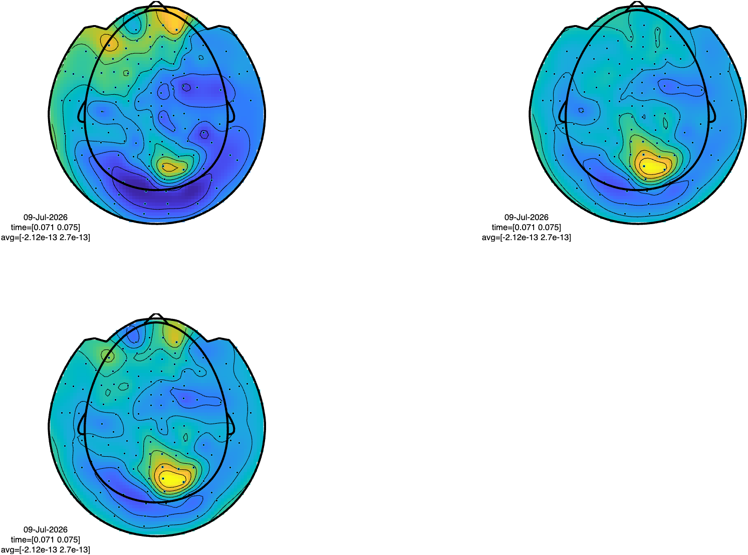
Now we can compare the result of the two different ways of cleaning by computing the ERF and displaying the results together
% compute ERF
cfg = [];
cfg.channel = 'MEG';
cfg.preproc.demean = 'yes';
cfg.preproc.baselinewindow = [-0.1 0];
tlck_ssp1 = ft_timelockanalysis(cfg, data_ssp1);
tlck_ssp2 = ft_timelockanalysis(cfg, data_ssp2);

cfg        = [];
cfg.layout = 'fieldlinebeta2bz_helmet.mat';
cfg.figure = 'subplot';
cfg.showlegend = 'yes';
ft_topoplotER(cfg, tlck, tlck_ssp1, tlck_ssp2);
Exercise
Explore the effect of the SSP by interactively selecting sensors from the topographies to display the time courses. Which approach do you think will preserve more neural signal? Why might using the emptyroom data for SSP estimation be advantageous or disadvantageous compared to using the task data itself?
cfg            = [];
cfg.channel    = 'MEG';
cfg.keeptrials = 'yes';
tlck_trials_ssp1 = ft_timelockanalysis(cfg, data_ssp1);
tlck_trials_ssp2 = ft_timelockanalysis(cfg, data_ssp2);

tlck_trials0 = tlck_trials_ssp1;
tlck_trials0.trial(:) = 0;

nrpt   = numel(data.trial);
design = [ones(1,nrpt) ones(1,nrpt)*2; 1:nrpt 1:nrpt];

cfg           = [];
cfg.method    = 'analytic';
cfg.statistic = 'depsamplesT';
cfg.design    = design;
stat_ssp1 = ft_timelockstatistics(cfg, tlck_trials_ssp1, tlck_trials0);
stat_ssp2 = ft_timelockstatistics(cfg, tlck_trials_ssp2, tlck_trials0);

cfg        = [];
cfg.layout = 'fieldlinebeta2bz_helmet.mat';
cfg.figure = 'subplot';
cfg.parameter = 'stat';
cfg.xlim   = [0.07 0.075];
cfg.showlegend = 'yes';
ft_topoplotER(cfg, stat, stat_ssp1, stat_ssp2);
Exercise
Explore the effect of the SSP by interactively selecting sensors from the topographies to display the time courses of the T-statistics. Which approach do you think will preserve more neural signal? Why might using the emptyroom data for SSP estimation be advantageous or disadvantageous compared to using the task data itself?
Denoising with HFC
Harmonic Field Correction (HFC) is specifically designed for OPM data to remove environmental noise by modeling the low spatial frequency components of the magnetic field, since these low spatial frequency components originate from a location far away from the sensor array:
% clean the data with HFC
cfg = [];
cfg.order = 2;
data_hfc = ft_denoise_hfc(cfg, data);
The ft_denoise_hfc function applies HFC denoising with a specified order (here, order 2). The order determines the complexity of the harmonic model used to represent the environmental noise.
HFC is particularly effective for removing spatially smooth environmental noise that affects all sensors. The order parameter controls the number of spherical harmonic functions used to model the noise. Higher orders can capture more complex noise patterns but may also remove neural signal.
Denoising with AMM
Adaptive Multipole Modelling (AMM) identifies and removes ambient artifacts in a two-step procedure. It applies a spatial model, using heuristics similar to HFC, followed a temporal filtering step, whereby residual signal components that are highly correlated with the ambient noise are removed on a segment-by-segment basis. Thus, strictly speaking, the spatial filter changes over time, making this technique similar in spirit to the tSSS algorithm:
% clean the data with AMM
cfg = [];
cfg.amm.thr = 1-1e-8;
data_amm = ft_denoise_amm(cfg, data);
The ft_denoise_amm function applies AMM with a threshold parameter that determines the correlation cutoff used to define noise components in the temporal filtering step. The lower this value, the more (potentially neural) signal will be removed.
Exercise
Compute the ERF for the HFC and AMM denoised data, and explore the result of the cleaning. If time and enthusiasm permits, you can also play around with the parameters of the cleaning (e.g. cfg.order for HFC and/or cfg.amm.thr for AMM), and evaluate the effect on the resulting ERFs. Consult the help section of the respective functions for more information.
Summary and suggested further reading
This tutorial demonstrated several denoising techniques for OPM data:
- Emptyroom analysis: Characterizing the noise environment is crucial for understanding what types of noise need to be addressed.
- SSP denoising: Effective for removing spatially structured noise components, with the option to use either the task data or emptyroom data for noise estimation.
- HFC denoising and AMM denoising: Denoising strategies that have a few more ‘knobs to tweak’
Each method has its strengths and weaknesses:
- SSP is good at removing consistent noise patterns and does not need sensor position information. Can be used in combination with emptyroom data but requires the sensors to be in the same position as during the measurements-of-interest. It also does not work for head-free OPM recordings with movements.
- HFC is effective for low spatial frequency noise but requires precise sensor position information for accurate modelling.
- AMM is effective in removing noise whose spatiotemporal profile changes over time but requires precise sensor position information and runs the risk of overfitting.
Further reading material about the denoising of OPM data:
- Interference suppression techniques for OPM-based MEG
- Theoretical advantages of a triaxial OPM-MEG system
- Noise and artifact suppression in SQUID and wearable OPM-MEG
- Optimal configuration of on-scalp OPMs with fixed channel counts
- DSSP
- SSS
See also these tutorials
- Coregistration of Optically Pumped Magnetometer (OPM) data
- Denoising OPM data
- Designing a custom 3D printed OPM helmet
- Using a MEG phantom for validation and OPM calibration
- Preprocessing of Optically Pumped Magnetometer (OPM) data
- Comparing MEG sensitivity maps for SQUID and OPM sensor arrays