workshop / hangzhou2026 / analysis /
Analysis of OPM-MEG data
Introduction
Traditional MEG systems use superconducting quantum interference devices (SQUIDs), which require expensive cryogenic cooling with liquid helium and involve placing the sensors at least 2 cm from the scalp. Optically pumped magnetometers (OPMs), a new generation of MEG, eliminate the need for cryogenic cooling, allowing sensors to be placed closer to the scalp. OPMs are small individual sensors that allow the researcher to choose where to place them over the head. These sensors are held in place by 3D-printed helmets, which can be customized for each subject.
Even though both the SQUID and the OPM systems detect the brain’s magnetic fields, their data analysis steps differ a bit. In this tutorial we explore the differences in preprocessing and coregistration between the two systems.
OPMs are flexible in their placement, allowing for new recording strategies. These new recording strategies lead to new data analysis strategies. For example, in this tutorial we use a small number of OPMs (32 sensors) and do sequential recordings in which we position them over different places over the scalp.
OPMs are magnetometers, as their name suggests. Magnetometers are more sensitive to environmental noise than gradiometers, which most SQUID systems have. Several data analysis algorithms to remove environmental noise have been proposed (see Seymour et al (2022) for more details). In this tutorial, we apply homogeneous field correction (HFC). HFC works better with a large number of sensors.
Unlike SQUID systems, which have standard coregistration strategies, OPMs don’t have a single coregistration standard. In this tutorial, we coregister the OPMs with the MRI using an optical 3D scanner which captures the participant’s facial features along with the OPM helmet (Zetter et al., 2019).
This tutorial combines the FieldTrip tutorials on preprocessing of OPM data and coregistration of OPM data. It does not cover follow-up analyses (like source reconstruction) which in principle should not differ from the SQUID follow-up analyses, or alternative coregistration methods, which are covered in the tutorial on coregistration of OPM data.
This hands-on session is the follow-up of the hands-on session on planning the acquisition of OPM-MEG data, in which we designed an OPM helmet, placed OPM sensors according to the extended 10-20 system, and computed the sensitivity of the resulting sensor array. In this session we analyze OPM-MEG data that was recorded with a different helmet design, namely the FieldLine smart helmet.
Background
In this tutorial we will use recordings made with 32 OPM sensors placed in an adult-sized “smart” helmet with a total of 144 slots. This helmet is called “smart” as each slot allows the sensor to slide in until it touches the head surface, regardless of the head size and shape. To limit head movements we mounted the helmet on a wooden plate located behind the subject chair.
To acquire a measurement for each of the 144 helmet slots, we divided the experiment into six runs. To maintain the participant’s head fixed between runs, we kept 9 sensors around the participant’s head fixed for all the runs. The remaining 23 sensors were moved to different helmet slots in each run to cover the whole scalp as homogeneously as possible.
Install and start FieldTrip
If you have not yet done so, install FieldTrip and start it with
restoredefaultpath
cd path_to_directory/fieldtrip-xxxxxxxx
addpath(pwd)
ft_defaults
The dataset used in this tutorial
The data for this tutorial was recorded with a 32-sensor FieldLine HEDscan v3 system with a so-called smart helmet. Each OPM sensor has one channel that measures the normal component of the magnetic field.
We perform a left median nerve stimulation experiment on a single participant in both the SQUID and the OPM system. We expect to find a dipole 20 ms post-stimulation in the right primary somatosensory area (Andersen & Dalal, 2021; Buchner et al., 1994).
The dataset can be downloaded from our download server.
Download the data
Download the content of the analysis directory from the download server, and cd into the analysis directory. The file paths used in this tutorial are relative to your current working directory. The data is organized according to the BIDS standard as follows:
sub-01/ses-anat
sub-01/ses-opm
sub-01/ses-squid
The directory sub-01/ses-anat/anat contains the anatomical MRI, sub-01/ses-opm/meg contains the six OPM recordings (in fif format) together with the optical 3D scan and the template of the FieldLine helmet, and sub-01/ses-squid/meg contains the SQUID recording (in the form of a CTF .ds directory) together with the Polhemus head shape.
Procedure
In this tutorial for the SQUIDs we will take the following steps:
- Define trials and read the data using ft_definetrial and ft_preprocessing
- Remove artifacts using ft_rejectvisual
- Compute the averaged ERFs using ft_timelockanalysis
- Visualize the results for all the channels with ft_multiplotER
- Plot the 2D sensor topography for a specified latency with ft_topoplotER
- Coregister the MRI with the SQUIDs using HPI coils and the Polhemus head shape with ft_volumerealign
- Plot the 3D sensor topography for a specified latency with ft_plot_topo3d
For the OPMs we will take the following steps:
- Define trials and read the data using ft_definetrial and ft_preprocessing
- Remove artifacts using ft_denoise_hfc and ft_rejectvisual
- Compute the averaged ERFs using ft_timelockanalysis
- Rename duplicate channels
- Append the data over the six runs using ft_appendtimelock
- Add NaNs to the missing channels
- Visualize the results for all the channels with ft_multiplotER
- Plot the 2D sensor topography for a specified latency with ft_topoplotER
- Coregister the MRI with the OPMs using an optical 3D scanner. For this several functions are used: ft_read_headshape, ft_meshrealign, ft_defacemesh, and ft_transform_geometry
- Append sensors from the six runs using ft_appendsens
- Plot the 3D sensor topography for a specified latency with ft_plot_topo3d
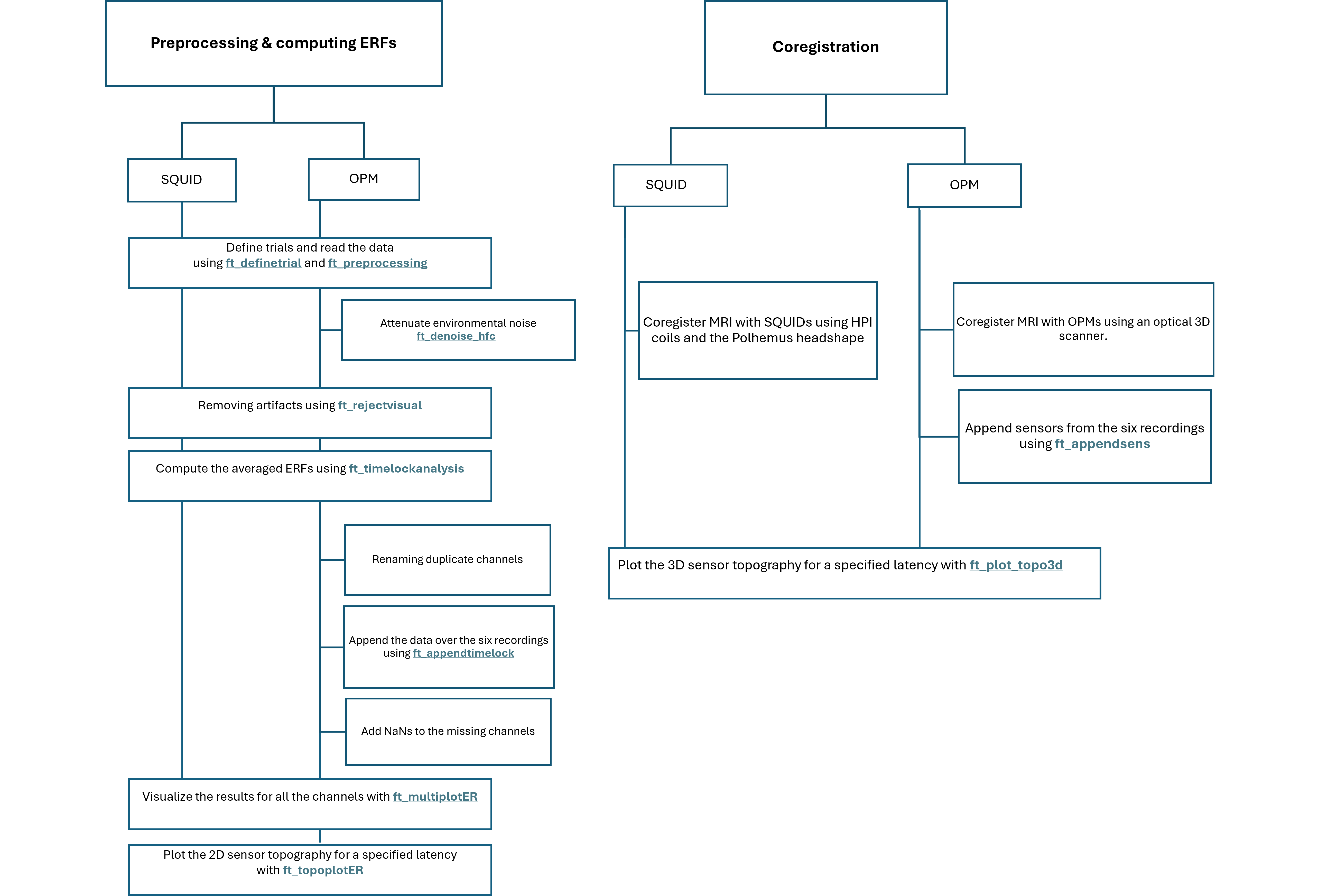
Preprocessing & computing ERFs
SQUID
We begin by reading the SQUID data and defining trials. We select trials in which left median nerve stimulation occurred (trigger code = 1). In the experiment, the inter-trial interval ranged from 800-1200 ms, so it makes sense to select a 200 ms prestimulus and 400 ms poststimulus window.
cfg                     = [];
cfg.dataset             = 'sub-01/ses-squid/meg/sub-01_ses-squid_task-MedianNervesStim_meg.ds';
cfg.trialdef.eventtype  = 'UPPT001';
cfg.trialdef.eventvalue = 1;
cfg.trialdef.prestim    = 0.2;
cfg.trialdef.poststim   = 0.4;
cfg                     = ft_definetrial(cfg);

cfg.demean         = 'yes'; % apply baseline correction
cfg.baselinewindow = [-Inf 0];
cfg.channel        = 'MEG';
cfg.continuous     = 'yes';
data_squid         = ft_preprocessing(cfg);
The summary method in ft_rejectvisual allows you to manually remove trials and/or channels that have high variance.
cfg              = [];
cfg.method       = 'summary';
data_squid_clean = ft_rejectvisual(cfg, data_squid);
We start by removing trials that have higher variance (bottom-left plot). Based on our data, a reasonable threshold to choose is 8e-25 Tesla-squared. Next, we assess the channel variance (top-right plot). Removing trials with high variance resulted in reducing the channel variance too, so no need to reject any channels.

We then calculate the ERFs:
cfg       = [];
avg_squid = ft_timelockanalysis(cfg, data_squid_clean);
We plot the activity from all the sensors.
cfg = [];
cfg.layout = 'CTF275_helmet';
ft_multiplotER(cfg, avg_squid); % use interactively
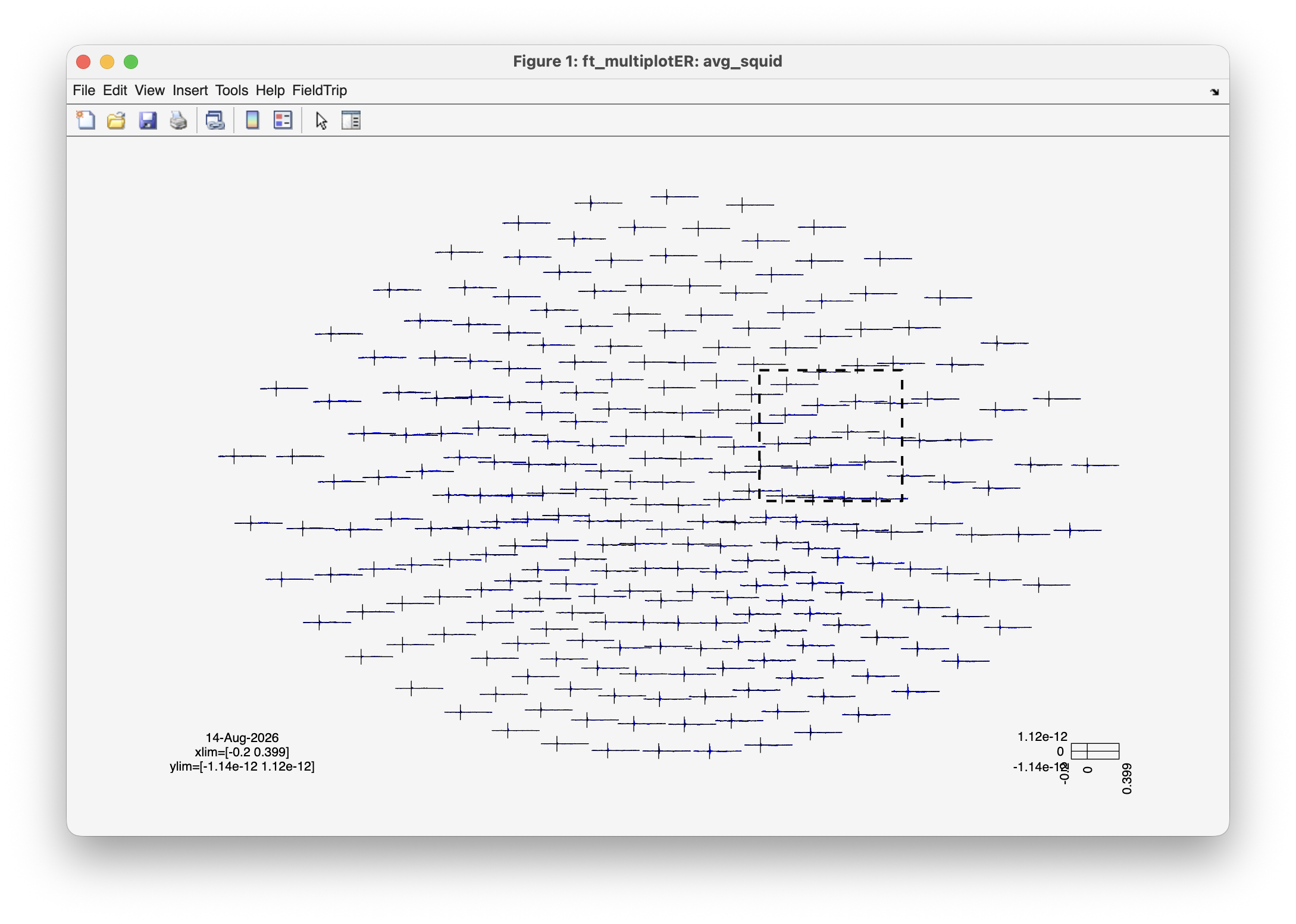
Interactive mode: Explore the event-related potential by dragging boxes around (groups of) sensors and time points in the ‘multiplot’ and the resulting ‘singleplots’ and ‘topoplots’. Can you find the time window that the dipolar activity at the right primary somatosensory area appears?
We can also plot this dipolar pattern with ft_topoplotER.
cfg = [];
cfg.xlim = [0.035 0.050];
cfg.layout = 'CTF275_helmet';
ft_topoplotER(cfg, avg_squid);

OPM
The OPM recordings are done sequentially over 6 runs, each corresponding to a single fif file.
d = dir('sub-01/ses-opm/meg/*.fif');

for i = 1:6 % 6 experimental runs
    cfg                     = [];
    cfg.dataset             = fullfile(d(i).folder, d(i).name);
    cfg.trialdef.eventtype  = 'ai61';
    cfg.trialdef.eventvalue = 1;
    cfg.trialdef.prestim    = 0.2;
    cfg.trialdef.poststim   = 0.4;
    cfg                     = ft_definetrial(cfg);

    cfg.demean         = 'yes'; % apply baseline correction
    cfg.baselinewindow = [-Inf 0];
    cfg.channel        = {'all', '-ai61'};
    data_opm(i)        = ft_preprocessing(cfg);
end

% save a copy to disk, as this step takes quite some time
save data_opm data_opm
OPMs are magnetometers, which are more sensitive to the environmental noise than the SQUID gradiometers. To remove some of the environmental noise, several algorithmic denoising techniques have been proposed (Seymour et al., 2022). In this tutorial we will apply homogeneous field correction (HFC) (Tierney et al., 2021).
for i = 1:6
    data_opm_nohdr(i) = rmfield(data_opm(i), 'hdr'); % this is needed so that FT_DENOISE_HFC works

    cfg               = [];
    data_opm_hfc(i)   = ft_denoise_hfc(cfg, data_opm_nohdr(i));
end
We will now manually remove trials with high variance.
for i = 1:6
    cfg                   = [];
    cfg.method            = 'summary';
    data_opm_hfc_clean(i) = ft_rejectvisual(cfg, data_opm_hfc(i));
end
Exercise
For the SQUID-based recordings, we removed trials with variance above the threshold of 8e-25 Tesla-squared. Is it possible to use the same threshold for the OPMs? If not, why and does this affect the quality of the OPM signal? Remember that (i) OPMs are magnetometers, and (ii) they are placed closer to the scalp than the SQUIDs.
for i = 1:6
    cfg        = [];
    avg_opm(i) = ft_timelockanalysis(cfg, data_opm_hfc_clean(i));
end
Before concatenating the six runs, we need to rename duplicate channels. Duplicates arise for three reasons: (i) 9 sensors remained fixed and were used across all runs, (ii) some sensors in the sixth run were in the same slot as the fifth run due to limited remaining free slots, and (iii) errors by the researcher placing a sensor in the same slot between runs. During the recording an Excel sheet was used to keep track in which slot each sensor was placed. We use that information to rename the channels.
avg_opm_rename = avg_opm;

% 9 sensors were fixed across all runs. Note that L101 was not working, so we do not need to rename it.
for k = 2:6
    index = find(ismember(avg_opm(k).label, {'R101_bz', 'L108_bz', 'R503_bz', 'L503_bz', 'L507_bz', 'R507_bz', 'R212_bz', 'L212_bz'})); % 2 in the back, 2 right, 2 left, 1 front, 1 top
    for i = 1:length(index)
        avg_opm_rename(k).label{index(i)} = strcat(avg_opm(k).label{index(i)}, '_', num2str(k));
    end
end

% some sensors in the sixth run were in the same slot as the fifth run
for k = 6 % 6th run
    index = find(ismember(avg_opm_rename(k).label, {'R114_bz', 'L504_bz'}));
    for i = 1:length(index)
        avg_opm_rename(k).label{index(i)} = strcat(avg_opm_rename(k).label{index(i)}, '_', num2str(k));
    end
end

% researcher's errors
for k = 2 % 2nd run
    index = find(ismember(avg_opm_rename(k).label, {'L214_bz'}));
    for i = 1:length(index)
        avg_opm_rename(k).label{index(i)} = strcat(avg_opm_rename(k).label{index(i)}, '_', num2str(k));
    end
end

for k = 5 % 5th run
    index = find(ismember(avg_opm_rename(k).label, {'R504_bz', 'L504_bz'}));
    for i = 1:length(index)
        avg_opm_rename(k).label{index(i)} = strcat(avg_opm_rename(k).label{index(i)}, '_', num2str(k));
    end
end
We concatenate the ERFs across the six runs to simulate a single experiment with 144 sensors (note: there are some missing sensors, so in the end we do not have 144 sensors).
cfg           = [];
cfg.appenddim = 'chan';
append_opm    = ft_appendtimelock(cfg, avg_opm_rename(1), avg_opm_rename(2), avg_opm_rename(3), avg_opm_rename(4), avg_opm_rename(5), avg_opm_rename(6));

% rename the appended average to "avg", as this is the default in FieldTrip
append_opm.avg = append_opm.trial;
append_opm     = rmfield(append_opm, 'trial');
There are some missing sensors. To avoid interpolation or extrapolation artifacts in the topography, we can add NaNs for the missing sensors and then tell ft_topoplotER to exclude those using the cfg.interpolatenan = 'no' option.
% read the layout of the FieldLine beta2 helmet with all 144 slots
cfg = [];
cfg.layout = 'fieldlinebeta2bz_helmet';
layout = ft_prepare_layout(cfg);

missing = setdiff(layout.label, append_opm.label);

% missing =
%
%   8x1 cell-array
%
%     {'L101_bz'}
%     {'L105_bz'}
%     {'L312_bz'}
%     {'L604_bz'}
%     {'R105_bz'}
%     {'R603_bz'}
%     {'R604_bz'}
%     {'R605_bz'}

% make a copy of the original timelock structure, remove two fields that we don't care about
append_opm_nan = rmfield(append_opm, {'dof', 'var'});

% add NaNs to the extra slots from the helmet that are missing
append_opm_nan.label = cat(1, append_opm_nan.label(:), missing(:));
append_opm_nan.avg   = cat(1, append_opm_nan.avg, nan(numel(missing), numel(append_opm_nan.time)));

cfg            = [];
cfg.layout     = 'fieldlinebeta2bz_helmet';
cfg.showlabels = 'yes';
cfg.ylim       = 'maxabs';
ft_multiplotER(cfg, append_opm_nan);

cfg                = [];
cfg.xlim           = [0.035 0.050];
cfg.layout         = 'fieldlinebeta2bz_helmet';
cfg.marker         = 'labels';
cfg.markerfontsize = 4;
cfg.zlim           = 'maxabs';
cfg.interpolatenan = 'no';
ft_topoplotER(cfg, append_opm_nan);

Exercise
Plot the topography including NaNs, then compare it with the topography where you excluded NaNs.
Coregistration
SQUID
We are now going to coregister the anatomical MRI to the SQUID coordinate system. We read the MRI, the SQUID channels and the Polhemus head shape in memory. We recommend converting all quantities to SI units to ensure consistent units throughout your pipeline.
mri    = ft_read_mri('sub-01/ses-mri/anat/sub-01_acq-mprage_T1w.nii');
ctf275 = ft_read_sens('sub-01/ses-squid/meg/sub-01_ses-squid_task-MedianNervesStim_meg.ds', 'senstype', 'meg');
shape  = ft_read_headshape('sub-01/ses-squid/meg/sub-01_ses-squid_headshape.pos');

mri    = ft_convert_units(mri, 'm');
ctf275 = ft_convert_units(ctf275, 'm');
shape  = ft_convert_units(shape, 'm');
To understand coregistration, you first need to know what coordinate systems are. Coregistration is about aligning data that is initially expressed in different coordinate systems into a single coordinate system.
Start by plotting the MRI, the SQUID sensors, and the Polhemus head shape to see in which coordinate systems these are expressed. You can use ft_determine_coordsys for that.
We coregister the MRI to the SQUIDs by converting the MRI coordinate system to match that of the SQUIDs. In other words, we ensure that the three fiducials (nasion, LPA and RPA) defined in the MRI coordinate system become aligned to the same three fiducials defined in the SQUID coordinate system.
% assign the 'ctf' coordinate system to the MRI
cfg              = [];
cfg.method       = 'interactive';
cfg.coordsys     = 'ctf'; % ALS coordinate system
mri_realigned1   = ft_volumerealign(cfg, mri);

% save mri_realigned1 mri_realigned1
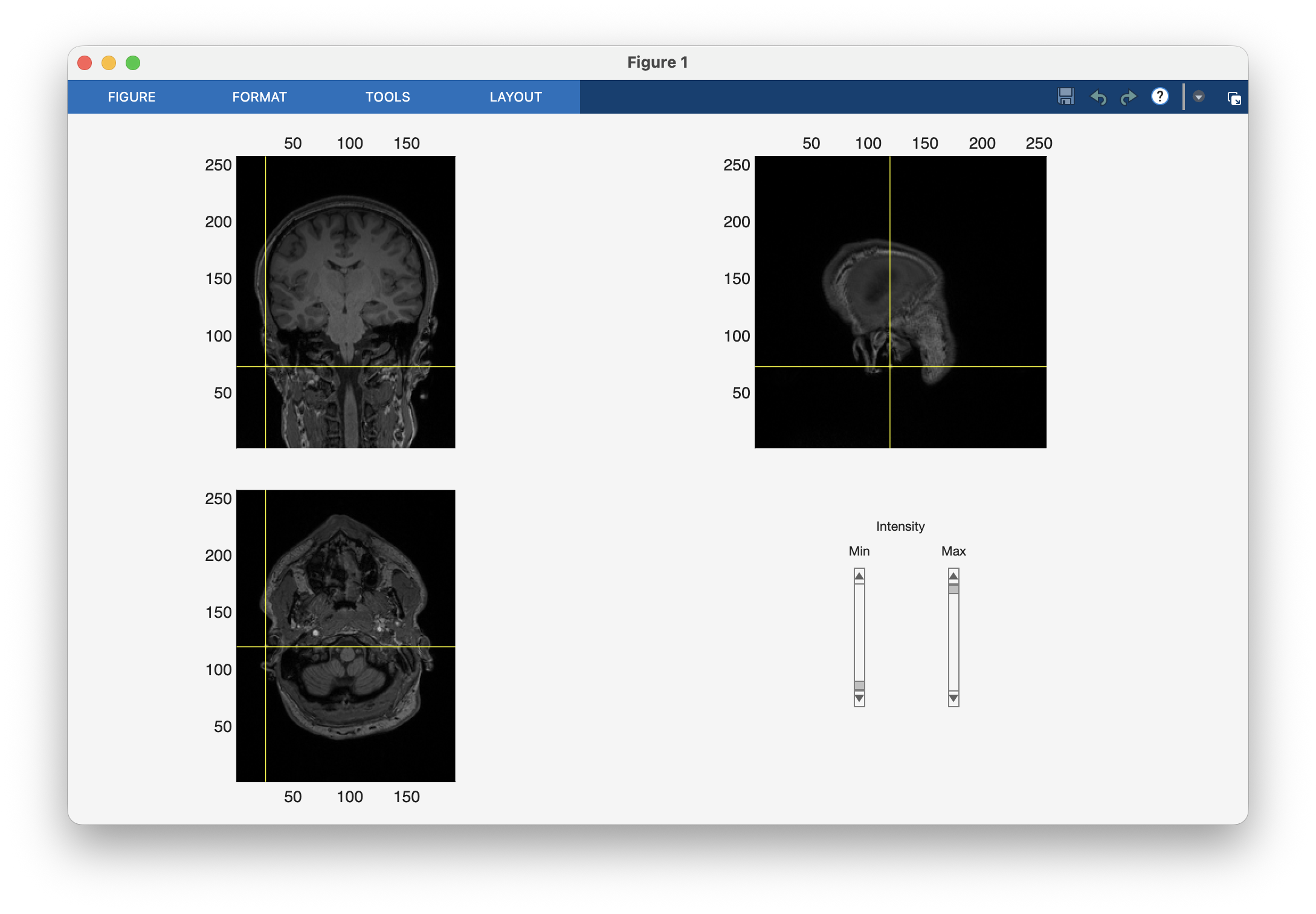
To refine the coregistration, we can also coregister the Polhemus head shape with the skin surface that is extracted from the previously aligned MRI. Now not only the fiducials but also other skin surface points acquired with the Polhemus are used for the alignment.
cfg = [];
cfg.method = 'headshape';
cfg.headshape.headshape = shape;
mri_realigned2 = ft_volumerealign(cfg, mri_realigned1);
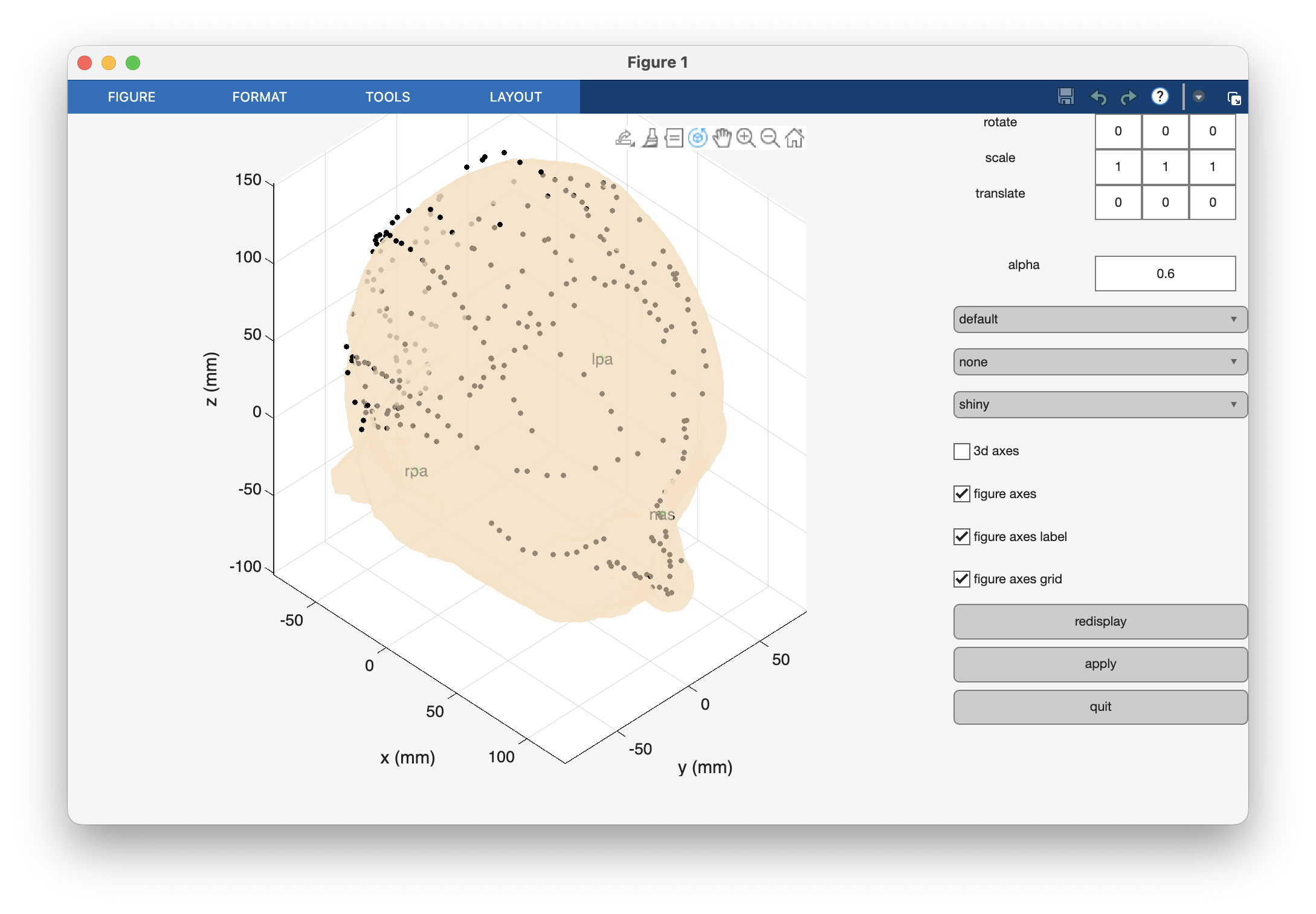
Although you can, you don’t have to make adjustments to the initial alignment. The alignment with the fiducials is a good starting point for the ICP.
% run once more to check
cfg = [];
cfg.method = 'headshape';
cfg.headshape.headshape = shape;
cfg.headshape.icp = 'no';
ft_volumerealign(cfg, mri_realigned2);

% save mri_realigned2 mri_realigned2
Let’s plot the sensor topography in 3D using ft_plot_topo3d. This will help us visualize where the sensors are positioned relative to the head. To make this clearer, we’ll also display the scalp and brain surfaces.
First, we’ll prepare the surface mesh of the scalp and brain:
cfg                = [];
cfg.output         = {'brain', 'scalp'};
mri_segmented      = ft_volumesegment(cfg, mri_realigned2);

% save it, we will reuse it later
save mri_segmented mri_segmented

cfg                = [];
cfg.tissue         = {'brain'};
mesh_brain         = ft_prepare_mesh(cfg, mri_segmented);

cfg                = [];
cfg.tissue         = {'scalp'};
mesh_scalp         = ft_prepare_mesh(cfg, mri_segmented);
Now, we’ll plot the 3D sensor topography for the time window [0.035, 0.050] seconds, along with the brain and scalp:
% do not select the reference sensors
index  = startsWith(ctf275.label, 'M');
pos275 = ctf275.chanpos(index, :);

% average the activity of interest in the time window [0.035 0.050] sec
t1 = nearest(avg_squid.time, 0.035);
t2 = nearest(avg_squid.time, 0.050);

selected_avg = mean(avg_squid.avg(:, t1:t2), 2);

% plot
figure
ft_plot_mesh(mesh_scalp, 'facealpha', 0.5, 'facecolor', 'skin', 'edgecolor', 'none', 'axes', true)
hold on
ft_plot_mesh(mesh_brain, 'facecolor', 'brain', 'edgecolor', 'none')
hold on
ft_plot_topo3d(pos275, selected_avg, 'facealpha', 0.9)
ft_headlight
view([90 0])

OPM
We will coregister the OPMs with the MRI using a scan from an optical 3D scanner which captures the participant’s facial features along with the OPM helmet. First we read and plot the optical scan:
scan      = ft_read_headshape('sub-01/ses-opm/meg/sub-01_ses-opm_opticalscan.obj');
scan.unit = 'm'; % assign the correct unit

figure
hold on
ft_plot_headshape(scan);
ft_plot_axes(scan);
lighting gouraud
material dull
light
We assign an initial coarse head-based coordinate system to the 3D scan, using the fiducial method in which we click on the nasion, LPA and RPA in the displayed scan.
cfg          = [];
cfg.method   = 'fiducial';
cfg.coordsys = 'neuromag';
scan_aligned = ft_meshrealign(cfg, scan);

% save scan_aligned scan_aligned

figure
hold on
ft_plot_headshape(scan_aligned);
ft_plot_axes(scan_aligned);
view([125 10]);
lighting gouraud
material dull
light
We remove irrelevant parts such as the body and cables. We use the ft_defacemesh function with a bounding box to keep only the desired head area.
cfg           = [];
cfg.method    = 'box';
cfg.selection = 'inside';
scan_head     = ft_defacemesh(cfg, scan_aligned);

% save scan_head scan_head
For “rotate” you specify [-30, 0, 0], for scale [0.2, 0.3, 0.2], and for translate [0, 40, 20]. Then you press “quit”.
figure
hold on
ft_plot_headshape(scan_head, 'axes', true);
view([125 10]);
lighting gouraud
material dull
light

We isolate the face region from the 3D scan using a bounding box. We will later align this face with the face extracted from the MRI.
cfg           = [];
cfg.method    = 'box';
cfg.selection = 'inside';
scan_face     = ft_defacemesh(cfg, scan_head);

% save scan_face scan_face

figure
hold on
ft_plot_headshape(scan_face, 'axes', true);
view([125 10]);
lighting gouraud
material dull
ft_headlight

We load the MRI. As the same participant took part in both the SQUID and the OPM recordings, we can reuse the segmented MRI from the SQUID analysis to save time:
load mri_segmented % from the SQUID analysis
We align the face from the 3D scan with the face extracted from the MRI.
% create a mesh for the scalp
cfg             = [];
cfg.tissue      = 'scalp';
cfg.numvertices = 10000;
mri_face        = ft_prepare_mesh(cfg, mri_segmented);

% alignment
cfg               = [];
cfg.method        = 'interactive';
cfg.headshape     = mri_face;
cfg.meshstyle     = {'edgecolor', 'k', 'facecolor', 'skin'};
scan_face_aligned = ft_meshrealign(cfg, scan_face);

% save scan_face_aligned scan_face_aligned

figure
hold on
ft_plot_headshape(mri_face, 'facealpha', 0.4);
ft_plot_mesh(scan_face_aligned, 'facecolor', 'skin');
view([125 10]);
lighting gouraud
material dull
ft_headlight

We align the whole head (including helmet) from the 3D scan with the reference helmet. For this we use the 3D model of the actual FieldLine helmet. The reference helmet only contains the rim around the face.
helmet_rim = ft_read_headshape('sub-01/ses-opm/meg/fieldlinebeta2_helmet_rim.mat');

cfg                   = [];
cfg.method            = 'interactive';
cfg.headshape         = helmet_rim;
cfg.meshstyle         = {'edgecolor', 'none', 'facecolor', [1 0.5 0.5]};
scan_helmet_aligned   = ft_meshrealign(cfg, scan_head);

% save scan_helmet_aligned scan_helmet_aligned

figure
hold on
ft_plot_mesh(helmet_rim, 'edgecolor', 'none', 'facecolor', [0.5 0.5 1], 'facealpha', 0.4);
ft_plot_mesh(scan_helmet_aligned, 'edgecolor', 'none', 'facecolor', [1 0.5 0.5], 'facealpha', 0.4);
view([145 10]);
lighting gouraud
material dull
ft_headlight

The three objects (the optical 3D scan, the face from the MRI and the template helmet) are initially all expressed in different coordinate systems. In the previous steps we have determined two pairwise transformations, which can be combined and used to align each of the objects to any other object.
Now we can use the transformation that aligns the face from the 3D scan with the face from the anatomical MRI and the transformation that aligns the helmet from the 3D scan with the reference helmet to calculate the transformation that aligns the reference helmet with the anatomical MRI.
transform_scan2helmet = scan_helmet_aligned.cfg.transform;
transform_scan2face   = scan_face_aligned.cfg.transform;
transform_helmet2face = transform_scan2face/transform_scan2helmet;
The transformation matrix transform_helmet2face can now be used to coregister the OPM sensors with the MRI, which aligns the OPM sensors with the head-based coordinate system. Before applying the transformation, we need to read the OPM sensors from the six fif files and combine them into a single sensor structure. In the FieldLine system the OPM sensors slide into the smart helmet; the fif file contains the actual position of the sensors relative to the helmet.
d = dir('sub-01/ses-opm/meg/*.fif');

for i = 1:6
    sensfile = fullfile(d(i).folder, d(i).name);
    grad_opm(i)  = ft_read_sens(sensfile);
end

% save grad_opm grad_opm

cfg               = [];
grad_opm_combined = ft_appendsens(cfg, grad_opm(1), grad_opm(2), grad_opm(3), grad_opm(4), grad_opm(5), grad_opm(6)); % removes the duplicate channels

% save grad_opm_combined grad_opm_combined
We apply the transformation to align the OPM sensors with the head-based coordinate system.
fieldlinebeta2_head = ft_transform_geometry(transform_helmet2face, grad_opm_combined);

% save fieldlinebeta2_head fieldlinebeta2_head

figure
hold on
ft_plot_sens(fieldlinebeta2_head, 'label', 'off');
ft_plot_headshape(mri_face, 'facecolor', [0.5 0.5 1], 'facealpha', 0.8, 'edgecolor', 'none');
view([125 10]);
lighting gouraud
material dull
ft_headlight

The alignment here is not optimal yet, the sensors are not on the scalp. Ideally, the model for the sensors should hover uniformly 5 mm above the scalp, since the sensitive pickup point from each sensor is 5 mm from its bottom.
Lastly, we plot the 3D sensor topography for the time window from 35 to 50 ms, along with the scalp:
[i_avg, i_sens] = match_str(append_opm.label, fieldlinebeta2_head.label);

% average the activity of interest in the time window [0.035 0.050] sec
t1 = nearest(append_opm.time, 0.035);
t2 = nearest(append_opm.time, 0.050);

selected_avg = mean(append_opm.avg(:, t1:t2), 2);

% plot
figure
ft_plot_mesh(mesh_scalp, 'facealpha', 0.2, 'facecolor', 'skin', 'edgecolor', 'none')
hold on
ft_plot_topo3d(fieldlinebeta2_head.chanpos(i_sens, :), selected_avg(i_avg), 'facealpha', 1)
ft_headlight
view([90 0])

Why do you think there’s a gap on the right side of the topography? Hint: Interpolation.
How do the 3D sensor topographies of OPMs and SQUIDs differ, and what causes these differences?
Summary and suggested further reading
In this tutorial we analyzed OPM-MEG data from a left median nerve stimulation experiment, and we compared the preprocessing and coregistration steps with those for the same experiment recorded with a SQUID system. For the OPMs we removed environmental noise with HFC, and we combined the six sequential runs into a single virtual experiment with almost 144 sensors by renaming the duplicate channels, appending the data over the runs and adding NaNs for the missing sensors. We coregistered the OPMs with the anatomical MRI using an optical 3D scan of the participant’s face and helmet, combined the transformations to express the OPM sensors in the same coordinate system as the MRI, and plotted the 3D sensor topographies of the somatosensory evoked field for both the OPM and the SQUID system.
See also
For more information, see also the following tutorials:
- Coregistration of Optically Pumped Magnetometer (OPM) data
- Denoising OPM data
- Designing a custom 3D printed OPM helmet
- Using a MEG phantom for validation and OPM calibration
- Preprocessing of Optically Pumped Magnetometer (OPM) data
- Comparing MEG sensitivity maps for SQUID and OPM sensor arrays
and the following examples: