ChildBrain pre-conference workshop in Leuven, Belgium

By whom: Raul Granados, Simon Homölle
When: Tuesday 5 February 2019
Where: Pre-conference training courses at the ChildBrain conference in Leuven
Local organization: Raul Granados.

Program

09:00-09:15	Welcome
09:15-10:15	Lecture
10:15-10:30	Coffee break
10:45-12:00	Hands on

How should you prepare for the workshop?

For the hands on session, we kindly require you to bring a functional laptop with MATLAB and FieldTrip installed. This session will be divided in a theoretical introduction, followed by the practical session, for which we ask you to read the points below:

We expect that you know the basics of MATLAB and that you already have experience with MEG/EEG preprocessing and analysis.
As the focus is on source reconstruction, topics that will NOT be covered in great detail are segmenting, artifact handling, averaging, frequency and time-frequency analysis, statistics.
If you are not familiar with MATLAB or are not certain about your MATLAB skills, please go through the “MATLAB for psychologists” tutorial on http://www.antoniahamilton.com/matlab.html.
To understand the FieldTrip toolbox design, please read the FieldTrip reference paper.
We will not spend too much time on understanding how MATLAB works and how FieldTrip organizes the data. Therefore if you have never done any FieldTrip analysis in MATLAB before, you should read this introduction tutorial.

In the hands-on session we will start with preprocessing structural MRI data, but will not spend too much time on understanding how MATLAB works and how FieldTrip organizes the data. Therefore if you have never done any FieldTrip analysis in MATLAB before, you should read this introduction tutorial. We will start at 9:00 sharp and will finish around 12:00.

Setting up for the hands-on session

To get going, you need to start MATLAB. Then, you need to issue the following command

restoredefaultpath
cd <path_to_fieldtrip>
addpath(pwd)
ft_defaults

global ft_default
ft_default.spmversion = 'spm12';

Please do NOT use the graphical path management tool from MATLAB. In this hands-on session we’ll manage the path from the command line, but in general you are much better off using the startup.m file than the path GUI.

Please do NOT add FieldTrip with all subdirectories, subdirectories will be added automatically when needed, and only when needed.

The restoredefaultpath command clears your path, keeping only the official MATLAB toolboxes. The addpath(pwd) statement adds the present working directory, i.e. the directory containing the FieldTrip main functions. The ft_defaults command ensures that all required subdirectories are added to the path. Setting the spmversion in the global ft_default variable ensures that all FieldTrip functions will use SPM12 rather than an older SPM version which sometimes causes issues with the mex files.

If you get the error “can’t find the command ft_defaults” you should check the present working directory.

After installing FieldTrip to your path, you need to change into the hands-on specific directory, containing the data that is necessary to run the specific hands-on session. These folders are located in C:\FieldTrip_workshop\.

Introduction

The aim of this tutorial is to create a head model of an adolescent with the numerical method of the Boundary Element Method (BEM), and if as an additional task with the Finite Element Method (FEM). The John E. Richards Lab provided us with an example MRI which consists of the averaged MRI of several 14 year old subjects.

Background

The EEG/MEG signals measured on or around the scalp do not directly reflect the activated neurons in the brain. To reconstruct the actual activity in the brain, source reconstruction techniques are used. You can read more about the different methods in the review papers that are listed here.

The activity in the brain is estimated from the EEG or MEG signals using

the EEG/MEG activity itself that is measured on or around the scalp
the spatial arrangement of the electrodes/gradiometers relative to the brain (sensor positions),
the geometrical and conductive properties of the head (head model)
the location of the source (source model)

Using this information, source estimation comprises two major steps: (1) Estimation of the EEG potential or MEG field distribution for a known source is referred to as forward modeling. (2) Estimation of the unknown sources corresponding to the measured EEG or MEG is referred to as inverse modeling.

The forward solution can be computed when the head model, the sensor positions and a model for the source are given. For distributed source models and for scanning approaches such as beamforming, the source model consists of a discrete description of the the brain volume or of the cortical sheet in many voxels or vertices. When the forward solution is computed, the lead field matrix (with dimensions Nchan * Nsources) is calculated for each point, taking into account the head model and the sensor positions.

A prerequisite of forward modeling is that the geometrical description of the sensor positions, head model and source model are expressed in the same coordinate system (e.g., CTF, MNI, Talairach) and with the same units (mm, cm, or m). There are different conventions for coordinate systems. The precise coordinate system is not relevant, as long as all data is consistent. Here you can read how the different head and MRI coordinate systems are defined. For most MEG systems, the gradiometers are by default defined relative to head localizer coils or anatomical landmarks, therefore when the anatomical MRI are aligned to the same landmarks, the position of the MEG sensors directly matches the MRI. As EEG data is typically not explicitly aligned relatively to the head, therefore, the EEG electrodes usually have to be explicitly realigned prior to source reconstruction (see also this faq and this example).

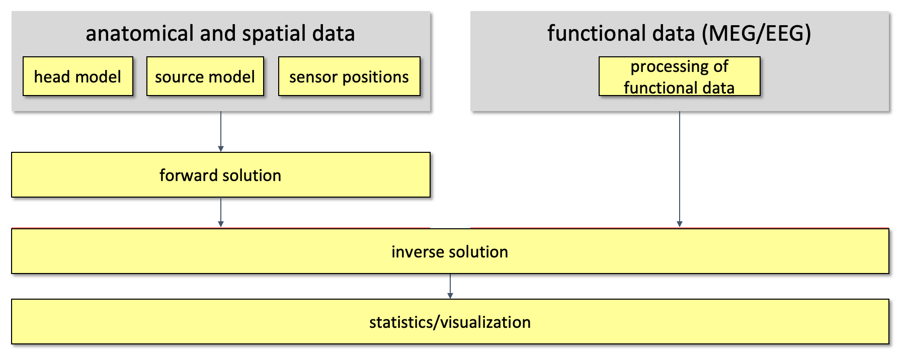
Figure 1. Overall outline of the pipeline used for source reconstruction

Procedure

As already mentioned, the goal of this session is to solve the EEG forward problem, more precisely we want to compute EEG leadfields so that the inverse problem can be solved. In order to compute leadfields, there are 9 main steps that have to be followed.

Load and read the anatomical data (ft_read_mri);
Align the MRI to the CTF coordinates. (ft_volumerealign);
Reslice the MRI image so that the voxels of the anatomical data are homogeneous (i.e. the size of the voxel is the same into each direction). This step will facilitate the segmentation step. (ft_volumereslice)
Segment the MRI: 3 compartments (scalp, skull, brain) (ft_volumesegment);
then we create the mesh: triangulated surface mesh for BEM and hexahedral volume mesh for FEM (ft_prepare_mesh).
Create the head models (headmodel_bem) where geometrical and electrical information are merged together (ft_prepare_headmodel);
Align the electrodes to the head surface (ft_electroderealign);
The source model is created, where the location of the sources is restrained to the brain compartment (from the BEM mesh) (ft_prepare_sourcemodel);
Leadfields can be computed (ft_prepare_leadfield).

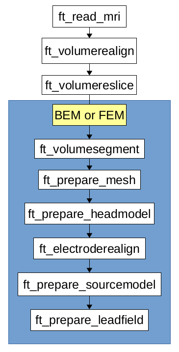
Figure 1: Pipeline for forward computation, in the blue box there are the steps which differ between BEM and FEM

1. Read the MRI

First of all we have to load the data

mri_orig = ft_read_mri('ANTS14-0Years3T_head_bias_corrected.nii');

Visualize the MRI

cfg = [];
ft_sourceplot(cfg,mri_orig);

Figure 2: Visualization of the MRI

2. Realign the MRI

In this step we will interactively align the MRI to the CTF space. We will be asked to identify the three CTF landmarks + zpoint (nasion, NAS; right pre-auricular point, RPA; left pre-auricular point, LPA) in the MRI. The zpoint is a point in the upper part of the head, it only serves to make sure that coordinate system is not upside down. It is important that all geometrical is expressed in the same coordinate system. This helps for coregistration of these data.

cfg = [];
cfg.method   = 'interactive';
cfg.coordsys = 'ctf';
mri_realigned = ft_volumerealign(cfg, mri_orig);

We can visualize the realigned MRI

cfg = [];
ft_sourceplot(cfg, mri_realigned);

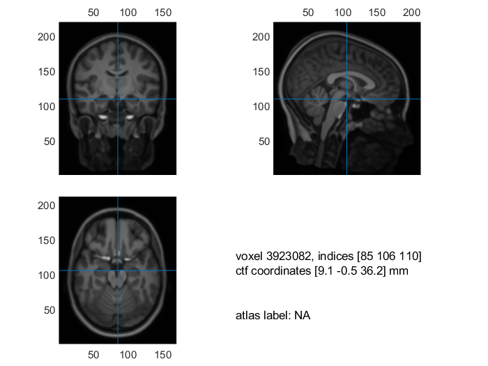
Figure 3: Visualization of the realigned MRI

3. Reslice the MRI

Before we segment the MRI, we will first reslice the MRI. The reason why is that a segmentation works properly when the voxels of the anatomical images are homogenous.

cfg = [];
mri_resliced = ft_volumereslice(cfg, mri_realigned);

We can visualize the resliced MRI

cfg = [];
ft_sourceplot(cfg, mri_resliced);

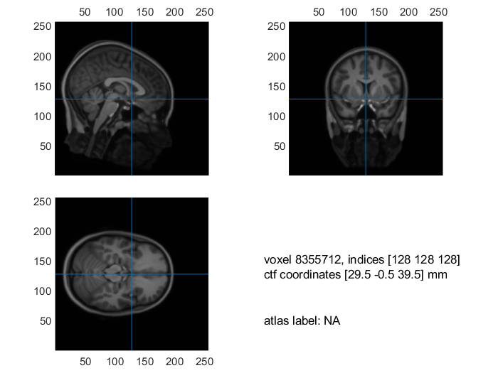
Figure 3: Visualization of the realigned MRI

4. Segment the MRI

Now we can segment the 3 different tissues we are interested in for our head model

cfg = [];
cfg.output = {'brain','skull', 'scalp'};
mri_segmented_3_compartment = ft_volumesegment(cfg, mri_resliced);

save mri_segmented_3_compartment mri_segmented_3_compartment

Visualize the segmentation

seg_i = ft_datatype_segmentation(mri_segmented_3_compartment,'segmentationstyle','indexed');

cfg = [];
cfg.funparameter = 'seg';
cfg.funcolormap  = gray(4); % distinct color per tissue
cfg.location     = 'center';
cfg.atlas        = seg_i;
ft_sourceplot(cfg, seg_i);

Figure 4: 3 compartment segmentation output

5. Create the mesh

On the basis of the segmentation we can now create a geometrical description of the head as a mesh

cfg = [];
cfg.tissue      = {'brain','skull','scalp'};
cfg.numvertices = [3000 2000 1000];
mesh_bem = ft_prepare_mesh(cfg,mri_segmented_3_compartment);

Visualize the mesh

figure, ft_plot_mesh(mesh_bem(1),'surfaceonly','yes','vertexcolor','none','facecolor',...
           'skin','facealpha',0.5,'edgealpha',0.1)
ft_plot_mesh(mesh_bem(2),'surfaceonly','yes','vertexcolor','none','facecolor',...
           'skin','facealpha',0.5,'edgealpha',0.1)
ft_plot_mesh(mesh_bem(3),'surfaceonly','yes','vertexcolor','none','facecolor',...
           'skin','facealpha',0.5,'edgealpha',0.1)

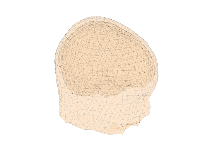
Figure 5: 3 compartment mesh with electrodes

6. Create the head model

Now we are ready and to create the a head model on the basis of the mesh.

cfg = [];
cfg.method = 'dipoli'; % You can also specify 'bemcp', or another method.
headmodel_bem = ft_prepare_headmodel(cfg, mesh_bem);

In Windows the method ‘dipoli’ does not work. You can explore other BEM method like ‘bemcp’. If you use ‘bemcp’, the conductivity field has a different order: {‘brain’, ‘skull’, ‘skin’}.

7. Align the electrodes

First we have to load a suitable electrode set. For this tutorial we will load a template dataset and transform it in such a way that it will fit the head surface.

elec = ft_read_sens('standard_1020.elc');

And now we will fit it to the head surface.

cfg = [];
cfg.method    = 'interactive';
cfg.elec      = elec;
cfg.headshape = headmodel_bem.bnd(3);
elec = ft_electroderealign(cfg);

Check the alignment visually.

figure;
ft_plot_axes(mesh_bem(1))
hold on;
ft_plot_mesh(mesh_bem,'surfaceonly','yes','vertexcolor','none','facecolor',...
           'skin','facealpha',0.5,'edgealpha',0.1)
ft_plot_sens(elec,'style', '.k');

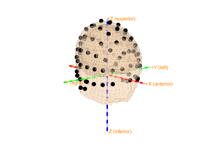
Figure 6: Mesh, electrodes and axes.

8. Create the source model

Before we are able to create the leadfields

cfg = [];
cfg.resolution = 7.5;
cfg.threshold       = 0.1;
cfg.smooth          = 5;
cfg.headmodel       = headmodel_bem;
cfg.inwardshift     = 1; % shifts dipoles away from surfaces
sourcemodel = ft_prepare_sourcemodel(cfg, headmodel_bem);

Visualize the source model

figure, ft_plot_mesh(sourcemodel.pos(sourcemodel.inside,:))
hold on, ft_plot_mesh(mesh_bem(1),'surfaceonly','yes','vertexcolor','none','facecolor',...
           'skin','facealpha',0.5,'edgealpha',0.1)

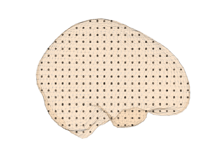
Figure 7: Sourcemodel on the brain compartment

Save the source model

save sourcemodel sourcemodel;

9. Compute the leadfield

We will now compute the lead field for every source in the source model.

cfg = [];
cfg.grid = sourcemodel;
cfg.headmodel  = headmodel_bem;
cfg.elec = elec;
leadfield_bem = ft_prepare_leadfield(cfg);

This is the last step for creating a forward model. We could now use the lead fields of each source to do the inverse modeling!

10. Further tasks

Exercise 1

So far we only created a BEM volume conduction model. To create a FEM volume conduction model use the same steps as beforehand.

Change Step 5 into

cfg = [];
cfg.tissue = {'brain','skull','scalp'};
cfg.method = 'hexahedral';
mesh_fem = ft_prepare_mesh(cfg,mri_segmented_3_compartment);

and Step 6 into

cfg = [];
cfg.method = 'simbio'; % Unfortunately this is not available on Windows.
headmodel_bem = ft_prepare_headmodel(cfg, mesh_bem);

Exercise 2

You can also find the segmentation ‘AVG14-0Years3T_segmented_BEM3.mat’ to create a head model. This a segmentation is processed version of a segmentation provided by alongside the MRI in the Neurodevelopmental MRI Database from the John E. Richards Lab. The segmentation was already preprocessed with the Steps 1-4.

Summary and Comments

This tutorial was about the creation of a volume conduction model on the basis of averaged MRIs of 14 year old subjects, creation of a source model, and computation of the lead fields. This head model could subsequently be used for source level analysis.