workshop / oxford2019 / sensor_analysis_plusminus /
Reading in data and performing sensor-level ERF and TFR analyses
This tutorial was written specifically for the workshop in Oxford in May 2019, and is a modified version of the sensor analysis tutorial. Specifically, a bit is added here about reading in data and preprocessing, and the bit about sensor-level connectivity analysis is removed.
Introduction
In this tutorial, we will provide an overview of several sensor-level analyses to help you get started working with FieldTrip. We will work on a dataset (Schoffelen, Poort, Oostenveld, & Fries (2011) Selective Movement Preparation Is Subserved by Selective Increases in Corticomuscular Gamma-Band Coherence. J Neurosci. 31(18):6750-6758) collected during an experiment where subjects were instructed to fixate on a screen. Each trial started with the presentation of a cue pointing either rightward or leftward. This cue indicated which hand the subject had to use for the trial’s response. Next, the subjects were instructed to extend both their wrists. After a baseline interval of 1s, an inward drifting grating was visually presented. Then, after an unpredictable delay, the stimulus changed speed, after which the subjects had to increase their wrist extension on the one cued side only. This experimental design is illustrated in Figure 1. Magneto-encephalography (MEG) data was collected using a 151-channel CTF system. Also, electromyography (EMG) data was collected from electrodes attached to the bilateral musculus extensor carpi radialis longus.

Figure 1: illustration of the experimental paradigm.
We will show you how data is typically read from disk in FieldTrip. Then, we will perform two types of analyses in this tutorial. We will start by looking at the event-related field (ERF) surrounding visual stimulus onset. Next, we will examine the induced oscillatory activity during the visual stimulation.
This tutorial only briefly covers the steps required to import data into FieldTrip and preprocess it. This is covered in more detail in the preprocessing tutorial, which you can refer to if you want more details. This tutorial also does not cover the details of the various options available for doing spectral analysis. Please refer to the time-frequency analysis tutorial for that.
Reading in raw data from disk
Preprocessing of MEG or EEG data refers to reading the data into memory, segmenting the data around interesting events such as triggers, temporal filtering, and optionally rereferencing in the case of EEG. The ft_preprocessing function takes care of all these steps, i.e., it reads the data and applies the preprocessing options.
There are largely two alternative approaches for preprocessing, which especially differ in the amount of memory required. The first approach is to read all data from the file into memory, apply filters, and subsequently cut the data into interesting segments. The second approach is to first identify the interesting segments, read those segments from the data file and apply the filters to those segments only. The remainder of this tutorial explains the second approach, as that is the most appropriate for large data sets such as the MEG data used in this tutorial. The approach for reading and filtering continuous data and segmenting afterwards is explained in another tutorial.
Preprocessing involves several steps including identifying individual trials from the dataset, filtering and artifact rejections. This tutorial covers how to identify trials using the trigger signal. Defining data segments of interest can be done
- according to a specified trigger channel
- according to your own criteria when you write your own trial function
This tutorial will focus on the first way, and briefly mention the second. Both ways depend on ft_definetrial. For more details, see the preprocessing tutorial.
The output of ft_definetrial is a configuration structure containing the field cfg.trl. This is a matrix representing the relevant parts of the raw datafile which are to be selected for further processing. Each row in the trl matrix represents a single epoch-of-interest, and the trl matrix has at least 3 columns. The first column defines (in samples) the beginpoint of each epoch with respect to how the data are stored in the raw datafile. The second column defines (in samples) the endpoint of each epoch, and the third column specifies the offset (in samples) of the first sample within each epoch with respect to timepoint 0 within that epoch.
We will demonstrate reading in data based on the localizer task for the experiment that was described at the start. The SubjectCMC.zip data is available from the download server. In this localizer task, a simple cue was presented 50 times, instructing the participant to lift the left or right wrist and keep the muscle contracted for 10 seconds. We will use the default trialfun ft_trialfun_general to define trials based on the triggers sent alongside these cues. We want to read in 1s of data before each trigger, and 10s of data after each trigger. This is achieved by the following:
cfg = [];
cfg.dataset = 'SubjectCMC.ds';
cfg.trialfun = 'ft_trialfun_general';
cfg.trialdef.eventtype = 'backpanel trigger'; % the name of your trigger channel
cfg.trialdef.eventvalue = 1:50; % which triggers to look for
cfg.trialdef.prestim = 1; % 1s of data before each trigger
cfg.trialdef.poststim = 10; % 10s of data after each trigger
cfg = ft_definetrial(cfg);
Note that we’re taking the output of ft_definetrial and storing it in our cfg variable. The output cfg now additionally has a field cfg.trl that contains our trial definition. Using the created trial definition, we can add some preprocessing options and read in the data:
% the following tells the reading functions that the data on disk is continuous and not already segmented
cfg.continuous = 'yes'; % see https://www.fieldtriptoolbox.org/faq/continuous/

cfg.channel = {'MEG' 'EMGlft' 'EMGrgt' 'EOG' 'ECG'};

% just to show that you can apply a lowpass filter while reading in data
cfg.lpfilter = 'yes';
cfg.lpfreq = 40;
cfg.lpfilttype = 'firws'; % windowed-sinc FIR filter

% and use data padding for the filtering
cfg.padding = 13; % pad our 11s-long trials to 13s before filtering
cfg.padtype = 'data'; % this is the default when reading from disk

data = ft_preprocessing(cfg);
Now you could start working with these localizer data.
Reading in preprocessed data from the main task
For the rest of this tutorial we will be focusing on the data that were recorded during the main experiment described above. These data were read in and preprocessed already for your convenience. Clear the localizer data from memory:
clear data
We will download subjectK.mat and load the already preprocessed data with the following command:
load subjectK
Loading this will give you two data structures in your workspace: data_left, containing the trials where the subjects had to respond with the left wrist; and data_right, where the right wrist was cued.
Take a look at one of the data structure
data_left =

       hdr: [1x1 struct]
     label: {153x1 cell}
      time: {1x140 cell}
     trial: {1x140 cell}
   fsample: 400
      grad: [1x1 struct]
       cfg: [1x1 struct]
sampleinfo: [140x2 double]
Most important for now are the trial, time, and label fields. The trial field contains the data for each trial as channel X time points matrices. The time field contains the time axis for each trial, and the label field contains the names of the channels in the data.
Plot the data for the first trial, 130th channel
plot(data_left.time{1}, data_left.trial{1}(130,:));
Which channel is the 130th channel?
Time point 0 in all trials corresponds to the onset of the visual stimulation. Trials end when the visual stimulus changed its speed, which is when the subject had to move their wrist (so the data for the actual movement is not in the trials). The visual stimulus speed change happened at an unpredictable time after t=0, so not all trials are the same length. To see this, plot some trials like this:
for k = 1:10
plot(data_left.time{k}, data_left.trial{k}(130,:)+k*1.5e-12);
hold on;
end
plot([0 0], [0 1], 'k');
ylim([0 11*1.5e-12]);
set(gca, 'ytick', (1:10).*1.5e-12);
set(gca, 'yticklabel', 1:10);
ylabel('trial number');
xlabel('time (s)');

Figure 1a: Some example trials, with time t=0 marked.
Event-related analysis
When analyzing EEG or MEG signals, the aim is to investigate the modulation of the measured brain signals with respect to a certain event. However, due to intrinsic and extrinsic noise in the signals - which in single trials is often higher than the signal evoked by the brain - it is typically required to average data from several trials to increase the signal-to-noise ratio (SNR). One approach is to repeat a given event in your experiment and average the corresponding EEG/MEG signals. The assumption is that the noise is independent of the events and thus reduced when averaging, while the effect of interest is time-locked to the event. The approach results in ERPs and ERFs for respectively EEG and MEG. Timelock analysis can be used to calculate ERPs/ERFs.
In FieldTrip, ERPs and ERFs are calculated by ft_timelockanalysis. For this particular dataset, we are interested in the ERF locked to visual stimulation. Since visual stimulation was the same in both the response-right and response-left conditions, we can combine the two data sets using ft_appenddata:
cfg  = [];
data = ft_appenddata(cfg, data_left, data_right);
Next, proceed to compute the ER
cfg                 = [];
cfg.channel         = 'MEG';
tl                  = ft_timelockanalysis(cfg, data);
Plotting the results
FieldTrip provides several options for visualizing the results of event-related analyses: ft_singleplotER, ft_multiplotER, and ft_topoplotER (see the plotting tutorial for an extensive introduction to your plotting options). In most cases, ft_multiplotER is the most convenient start, as it provides easy access to the other two visualization methods through the graphical user interface. Call it like this:
cfg                 = [];
cfg.showlabels      = 'yes';
cfg.showoutline     = 'yes';
cfg.layout          = 'CTF151_helmet.mat';
ft_multiplotER(cfg, tl);
Note that we request channel labels and head outline showing, and with a particular template layout corresponding to our MEG acquisition system. The output should look like this:

Figure 2: event-related field for each MEG sensor.
As you can see, the event-related field for each MEG sensor is displayed at a location corresponding to the approximate location of each sensor.
The nice thing about this multiplot is that it is interactive: it is possible to select sensors and view an average plot (corresponding to an ft_singleplotER) of those sensors. There seems to be an interesting deflection in the ERF around the left occipitoparietal sensors. Go ahead and select those, and click the selection box that comes up.

Figure 3: click the box to show the average of the selected sensors.
The plot that comes up shows a major deflection around 300m

Figure 4: average ERF for some left posterior sensors.
Again, you can select a time range and click it to bring up a topographical plot (ft_topoplotER) of the ERF averaged over the selected time window. Select the peak around 300ms and click it.

Figure 5: topographical representation of the ERF deflection around 300ms after visual stimulus onset.
Given that the CTF system uses axial gradiometers (i.e. detecting the magnetic gradient orthogonal to the scalp), what electrical dipole configuration would explain the observed field pattern in the above figure?
Feel free to click around a bit in the multi- and singleplots to explore the characteristics of the ERF.
Use the cfg.baseline option in ft_multplotER to correct the ERF for the baseline in the pre-stimulus interval.
The planar gradient
The CTF MEG system has (151 in this dataset, or 275 in newer systems) first-order axial gradiometer sensors that measure the gradient of the magnetic field in the radial direction, i.e. orthogonal to the scalp. Often it is helpful to interpret the MEG fields after transforming the data to a planar gradient configuration, i.e. by computing the gradient tangential to the scalp. This representation of MEG data is comparable to the field measured by planar gradiometer sensors. One advantage of the planar gradient transformation is that the signal amplitude typically is largest directly above a source, whereas with axial gradient the signal amplitude is largest away from the source.
We can compute the planar magnetic gradient using ft_megplanar, which gives us the planar gradient in the vertical and horizontal orientations. For visualization, and many subsequent analysis steps, these components need to be combined, which is implemented by ft_combineplanar. Since averaging is a linear operation, it does not matter if we convert the data to planar gradient before or after the call to ft_timelockanalysis. However, later on we will do frequency analysis, where the order does matter, so we will use the same order here. To compute the planar gradient and recompute the ERFs on this dataset:
cfg                 = [];
cfg.method          = 'template';
cfg.template        = 'CTF151_neighb.mat';
neighbours          = ft_prepare_neighbours(cfg, data);

cfg                 = [];
cfg.method          = 'sincos';
cfg.neighbours      = neighbours;
data_planar         = ft_megplanar(cfg, data);

cfg                 = [];
cfg.channel         = 'MEG';
tl_planar           = ft_timelockanalysis(cfg, data_planar);

cfg                 = [];
tl_plancmb          = ft_combineplanar(cfg, tl_planar);
Note that we create a ‘neighbours’ structure before calling ft_megplanar. This is required by ft_megplanar because the ‘sincos’ algorithm needs to know which channels are adjacent to one another. Plot the results again:
cfg                 = [];
cfg.showlabels      = 'yes';
cfg.showoutline     = 'yes';
cfg.layout          = 'CTF151_helmet.mat';
ft_multiplotER(cfg, tl_plancmb);
The order in which you do the combining the planar channels and averaging does matter, since the combining consists of a non-linear transform.
Please be advised that this might result in unexpected and undesirable effects due to different number of trials and/or due to baselining effects. In general we recommend to not use combined planar gradients for ERFs, unless you know what you are doing. See also this example.
Time-frequency analysis
Background
Oscillatory components contained in the ongoing EEG or MEG signal often show power changes relative to experimental events. These signals are not necessarily phase-locked to the event and will not be represented in event-related fields and potentials (Tallon-Baudry and Bertrand (1999)). The goal of this section is to compute and visualize event-related changes by calculating time-frequency representations (TFRs) of power. This will be done using analysis based on Fourier analysis and wavelets. The Fourier analysis will include the application of multitapers (Mitra and Pesaran (1999), Percival and Walden (1993)) which allow a better control of time and frequency smoothing.
Calculating time-frequency representations of power is done using a sliding time window. This can be done according to two principles: either the time window has a fixed length independent of frequency, or the time window decreases in length with increased frequency. For each time window the power is calculated. Prior to calculating the power one or more tapers are multiplied with the data. The aim of the tapers is to reduce spectral leakage and control the frequency smoothing.
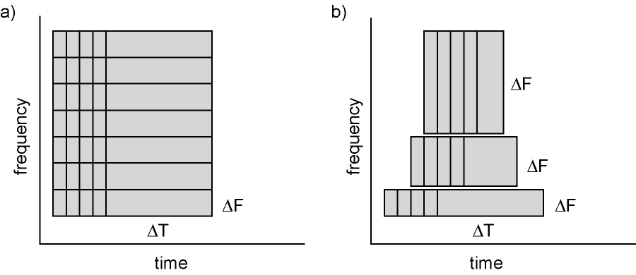
Figure 6: Time and frequency smoothing. (a) For a fixed length time window the time and frequency smoothing remains fixed. (b) For time windows that decrease with frequency, the temporal smoothing decreases and the frequency smoothing increases.
If you want to know more about tapers/ window functions you can have a look at this Wikipedia page. Note that Hann window is another name for Hanning window used in this tutorial. There is also a Wikipedia site about multitapers, to take a look at it click here.
Time-frequency representations using Hanning tapers
We will here describe how to calculate time frequency representations using Hanning tapers. When choosing for a fixed window length procedure the frequency resolution is defined according to the length of the time window (delta T). The frequency resolution (delta f in figure 1) = 1/length of time window in sec (delta T in figure 1). Thus a 500 ms time window results in a 2 Hz frequency resolution (1/0.5 sec= 2 Hz) meaning that power can be calculated for 2 Hz, 4 Hz, 6 Hz etc. An integer number of cycles must fit in the time window.
To compute our time-frequency representation (TFR), we will first subselect a piece of our trials using ft_redefinetrial. This is done to increase the speed at which the subsequent analysis will run. We need a part of the baseline interval and a part of the stimulation interval, so we choose the interval from -0.8s to 1.0s
cfg                 = [];
cfg.toilim          = [-0.8 1];
cfg.minlength       = 'maxperlen'; % this ensures all resulting trials are equal length
data_small          = ft_redefinetrial(cfg, data_planar);
The structure data_small contains less trials than the original data, because we want trials that last until at least 1s after stimulus onset. Recall that not all trials last that long, because the visual stimulus speed change might have happened before t=1s already. Note that we are again using the planar gradient data, in order to make interpreting the results easier. Now we move on to using ft_freqanalysis to compute our TFR using a 0.2s window size:
cfg                 = [];
cfg.method          = 'mtmconvol';
cfg.taper           = 'hanning';
cfg.channel         = 'MEG';

% set the frequencies of interest
cfg.foi             = 20:5:100;

% set the timepoints of interest: from -0.8 to 1.1 in steps of 100ms
cfg.toi             = -0.8:0.1:1;

% set the time window for TFR analysis: constant length of 200ms
cfg.t_ftimwin       = 0.2 * ones(length(cfg.foi), 1);

% average over trials
cfg.keeptrials      = 'no';

% pad trials to integer number of seconds, this speeds up the analysis
% and results in a neatly spaced frequency axis
cfg.pad             = 2;
freq                = ft_freqanalysis(cfg, data_small);
Again we have to combine the two components of the planar gradient
cfg                 = [];
freq                = ft_combineplanar(cfg, freq);
Plotting
Then we can plot the results using ft_multiplotTFR:
cfg                 = [];
cfg.interactive     = 'yes';
cfg.showoutline     = 'yes';
cfg.layout          = 'CTF151_helmet.mat';
cfg.baseline        = [-0.8 0];
cfg.baselinetype    = 'relchange';
cfg.zlim            = 'maxabs';
ft_multiplotTFR(cfg, freq);
Note the baseline and baselinetype parameters. These govern what baseline correction is applied to the data before plotting. In this case, we want to plot the relative change of our power data with respect to the interval between -0.8s and 0s (corresponding to the no-stimulation baseline interval in the experimental design).
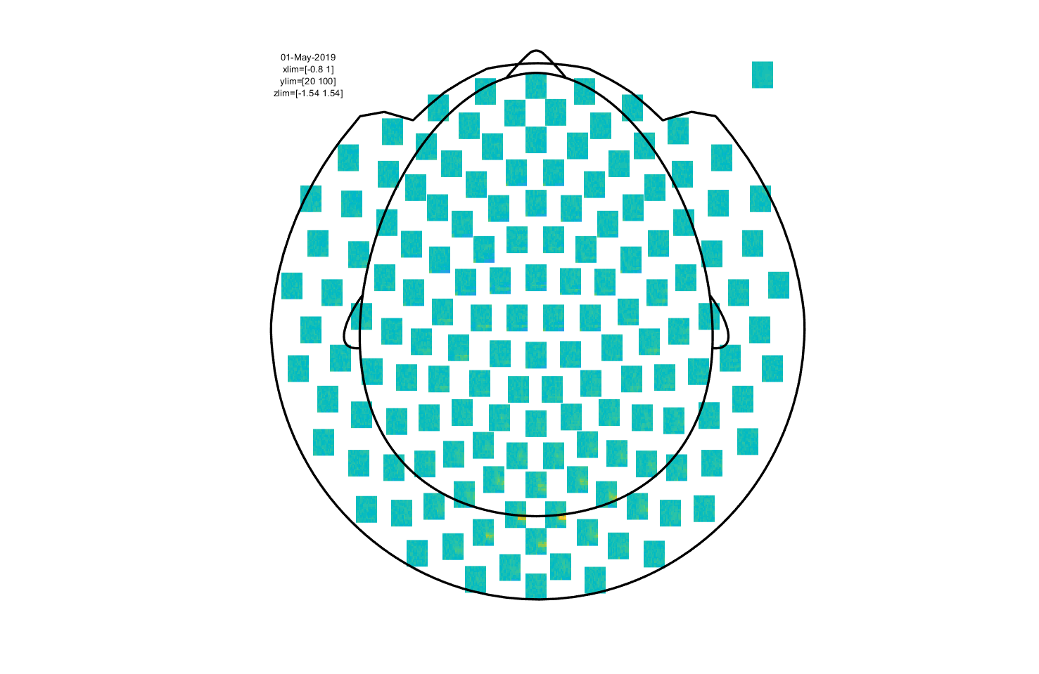
Figure 7: Time-frequency representation using a Hanning taper with a fixed window length.
This is an interactive plot, so just as with the event-related part you can select sensors and click to get an average TFR. With this, you can select a time and frequency range and plot a topography.
Click around the multiplot to explore the visual gamma response and its topography!
Overview of the conducted analysis
In a next step, you can get an overview of your analyses by clicking on the FieldTrip menu item and selecting “Show pipeline”:

Exactly the same can be achieved using ft_analysispipeline as follow
cfg = [];
ft_analysispipeline(cfg, freq);
The function ft_analysispipeline puts all conducted analysis steps into perspective and visualizes them in a flowchart:
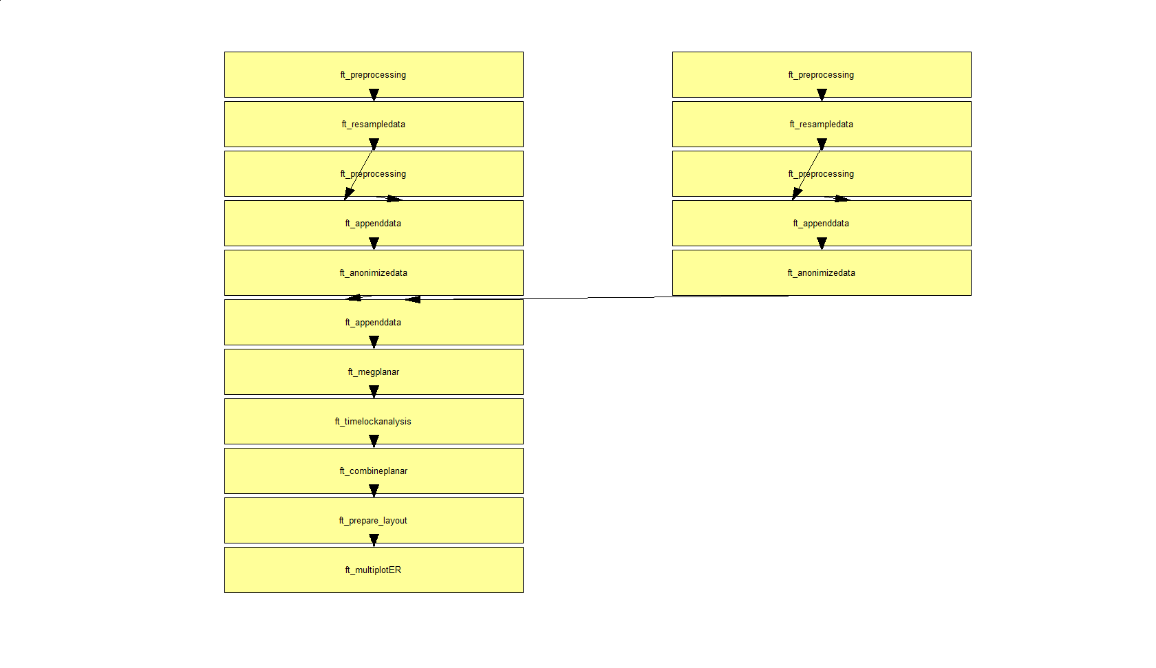
By clicking on one of the boxes (in MATLAB), a new figure will appear that shows all cfg-options that were used to in the respective function.
Summary and suggested further reading
This tutorial gave an overview of some options available in FieldTrip for doing sensor-level analysis. We started by showing how you can read data from disk using trigger channels and/or custom trial functions. Then, we investigated an event-related field evoked by visual stimulation and computed a planar gradient representation. Next, time-frequency analysis was performed and revealed induced visual gamma activity.
The tutorial on which this one was based contains an extra section on how to performance analysis of coherence of MEG signals with an external reference (in this case, EMG). If you’re done early, you may want to have a look at that one. It’s also a good basis for the tutorial we’ll later be doing on beamforming.
Alternatively, or additionally, you could read through the tutorial on time-frequency analysis, which provides more details on the various tapers available and their implications. Alternative follow-ups would be the tutorial on beamformers for source reconstruction (potentially the extended beamforming tutorial on the same data set as the present one) or, for details on statistics, one of the statistics tutorials.
See also these frequently asked questions
- How can I append the files of two separate recordings?
- How can I interpret the different types of padding in FieldTrip?
- How can I consistently represent artifacts in my data?
- Why should I start with rereferencing for BioSemi EEG data?
- Why should I set continuous to yes for CTF data?
- How can I convert one dataformat into an other?
- How can I read corrupted (unsaved) CTF data?
- What dataformats are supported?
- How can I import my own data format?
- Why is there a residual 50Hz line-noise component after applying a DFT filter?
- How can I deal with a discontinuous Neuralynx LFP recording?
- How can I read all channels from an EDF file that contains multiple sampling rates?
- What is the relation between "events" (such as triggers) and "trials"?
- How can I extend the reading functions with a new dataformat?
- Why am I not getting integer frequencies?
- How can I find out what eventvalues and eventtypes there are in my data?
- How can I merge two datasets that were acquired simultaneously with different amplifiers?
- I have problems reading in NeuroScan .cnt files. How can I fix this?
- How can I process continuous data without triggers?
- How can I preprocess a dataset that is too large to fit into memory?
- What kind of filters can I apply to my data?
- How does the filter padding in preprocessing work?
- How can I rename channels in my data structure?
- Do I need to resample my data, and if so, how is this to be done?
- Why does my TFR look strange (part I, demeaning)?
- Why does my TFR look strange (part II, detrending)?
- How can I check or decipher the sequence of triggers in my data?
- Reading is slow, can I write my raw data to a more efficient file format?
- How can I test whether a behavioral measure is phasic?
- In what way can frequency domain data be represented in FieldTrip?
- Does it make sense to subtract the ERP prior to time frequency analysis, to distinguish evoked from induced power?
- Why do I need to run ft_freqanalysis before ft_combineplanar?
- Why does my output.freq not match my cfg.foi when using 'mtmconvol' in ft_freqanalysis?
- Why does my output.freq not match my cfg.foi when using 'mtmfft' in ft_freqanalysis
- Why does my output.freq not match my cfg.foi when using 'wavelet' (formerly 'wltconvol') in ft_freqanalysis?
- Why am I not getting integer frequencies?
- What does "padding not sufficient for requested frequency resolution" mean?
- What convention is used to define absolute phase in 'mtmconvol', 'wavelet' and 'mtmfft'?
- How does mtmconvol work?
- What kind of filters can I apply to my data?
- How can I do time-frequency analysis on continuous data?
- Why does my TFR contain NaNs?
- Why does my TFR look strange (part I, demeaning)?
- Why does my TFR look strange (part II, detrending)?
- What is meant by time-frequency trade off?
- Why is the largest peak in the spectrum at the frequency which is 1/segment length?
See also these examples
- Use denoising source separation (DSS) to remove ECG artifacts
- Determine the filter characteristics
- Fixing a missing channel
- Independent component analysis (ICA) to remove ECG artifacts
- Independent component analysis (ICA) to remove EOG artifacts
- Combine MEG with Eyelink eyetracker data
- Getting started with reading raw EEG or MEG data
- Rereference EEG and iEEG data
- Detect the muscle activity in an EMG channel and use that as trial definition
- Making your own trialfun for conditional trial definition
- Common filters in beamforming
- Effect of SNR on Coherence
- Cross-frequency analysis
- Effects of tapering for power estimates
- Correlation analysis of fMRI data
- Fourier analysis of neuronal oscillations and synchronization
- Conditional Granger causality in the frequency domain
- Simulate an oscillatory signal with phase resetting
- Analyze steady-state visual evoked potentials (SSVEPs)
- Apply non-parametric statistics with clustering on TFRs of power that were computed with BESA