development / module / forward /
Forward computation of EEG/MEG source models
FieldTrip has a consistent set of low-level functions for forward computations of the EEG potential or MEG field. The spatial distribution of a known source in a volume conductor is called a leadfield.
The forward module comprises a complete toolbox of high-quality forward methods, i.e. it contains all functions to set up the volume conduction models of the head and to compute the leadfields. Using the high-level FieldTrip functions and the inverse module, these can be used for reconstructing the sources given real experimental MEG and EEG data.
The objective of supplying these low-level functions as a separate module/toolbox are to
- facilitate the reuse of these functions in other open source projects (e.g., EEGLAB, SPM)
- facilitate the implementation and support for new inverse methods, esp. for external users/contributors
- facilitate the implementation of advanced features
The low-level functions for source estimation/reconstruction are contained in the forward and inverse toolboxes, which are released together with FieldTrip. If you are interested in using them separately from the FieldTrip main functions, you can also download them separately here. For reference: in the past the forward and inverse modules were combined in a single “forwinv” toolbox.
Please note that if you are an end-user interested in analyzing experimental EEG/MEG data, you will probably want to use the high-level FieldTrip functions. The functions such as ft_preprocessing, ft_timelockanalysis and ft_sourceanalysis provide a user-friendly interface that take care of all relevant analysis steps and the data bookkeeping.
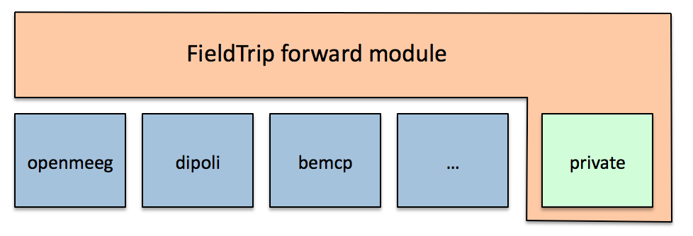
Module layout
The forward module contains functions with a user interface that will be easily understood by experienced programmers and methods developers and can be considered medium-level functions. They have a clear and consistent programming interface (API) which hides the specific details particular volume conduction models and that allows software developers to write forward methods without having to worry about integrating it with the inverse methods worry about data handling. The low-level functions on which the functions in the forward module depend are located in a private subdirectory which is not accessible from the MATLAB command line.
The forward module is complemented by an inverse module that contains the implementation of various high-quality inverse source estimation algorithms, such as dipole fitting, beamforming and linear estimation using the minimum-norm approach.
Instead of implementing all forward methods completely from scratch, the FieldTrip forward module makes use of some high quality implementations that have been provided by the original method developers. Some of these contributions consist of MATLAB code, some contain MEX files and some are implemented using an external command-line executable that is called from the command-line. All of these external implementations are fully wrapped in the FieldTrip forward module and do not require specific expertise on behalf of the end-user.
Supported methods for forward computations of the potential or field
The following forward methods are implemented for computing the electric potential (EEG)
- single sphere
- multiple concentric spheres with up to 4 shells
- boundary element model (BEM)
- leadfield interpolation using a precomputed grid
- all forward models supported by the Neuromag meg-calc toolbox
The following forward methods are implemented for computing the magnetic field (MEG)
- single sphere (Cuffin and Cohen, 1977)
- multiple spheres with one sphere per channel (Huang et al, 1999)
- realistic single-shell model based on leadfield expansion (Nolte, 2003)
- leadfield interpolation using a precomputed grid
Definition of the high-level function-calls (user interface)
Normally, end-users of the FieldTrip toolbox would use the functions in the main FieldTrip directory and not be calling the functions that are part of the forward module directly . The high-level FieldTrip functions characterize themselves by having a cfg argument as the first input, doing data handling, conversions of objects and try to support backward-compatibility with older end-user analysis scripts.
Some high-level functions FieldTrip functions that are of relevance for forward modeling are
- ft_read_mri and ft_read_sens
- ft_volumerealign, ft_volumereslice, and ft_volumesegment
- ft_electroderealign
- ft_prepare_mesh
- ft_prepare_headmodel, this calls ft_headmodel_xxx (see below)
- ft_prepare_leadfield, this calls ft_prepare_vol_sens and ft_compute_leadfield (see below)
In addition, there are some utility functions (residing in fieldtrip/utilities) that may be relevant, but which are not part of the module
These are explained in more detail in the appropriate tutorials.
Definition of the low-level function-calls (API)
Volume conduction models of the head are represented as a MATLAB structure, which content depends on the model details. In the subsequent documentation the volume conduction model structure is referred to as headmodel. The electrodes in case of EEG, or magnetometers or gradiometers in case of MEG, are described as a MATLAB structure. In the subsequent documentation this is referred to as elec for electrodes, grad for magnetometers and/or gradiometers, or sens to represent either electrodes or gradiometers.
Using the FieldTrip fileio module one can read in volume conduction models and the definition of the sensor array (electrodes or gradiometers) from file by using the ft_read_headmodel and/or ft_read_sens functions.
[headmodel] = ft_read_headmodel(filename)
[sens]      = ft_read_sens(filename)
This assumes that the volume conduction model was created in external software (e.g., CTF, Neuromag, or ASA) and that the sensor description is stored in an external acquisition-specific file format.
Alternative to reading the volume conduction model from an external file, you can of course also generate a volume conduction model based on a geometrical description of the head. For example, you can fit a single or multiple spheres to a set of points that describes the head surface. FieldTrip provides a separate function for the constructing of a head model for each of the EEG/MEG computational forward method
headmodel = ft_headmodel_asa(filename, ...)
headmodel = ft_headmodel_bemcp(geom, ...)
headmodel = ft_headmodel_concentricspheres(geom, ...)
headmodel = ft_headmodel_dipoli(geom, ...)
headmodel = ft_headmodel_duneuro(geom, ...)
headmodel = ft_headmodel_halfspace(location, orientation, ...)
headmodel = ft_headmodel_hbf(geom, ...)
headmodel = ft_headmodel_infinite(...)
headmodel = ft_headmodel_interpolate(filename, sens, sourcemodel, ...)
headmodel = ft_headmodel_localspheres(geom, grad, ...)
headmodel = ft_headmodel_openmeeg(geom, ...)
headmodel = ft_headmodel_simbio(geom, ...)
headmodel = ft_headmodel_singleshell(geom, sens, ...)
headmodel = ft_headmodel_singlesphere(pnt, ...)
Most of these functions take a geometrical description of the head, skull and/or brain surface as input. These geometrical descriptions of the shape of the head can for example be derived from an anatomical MRI, from a CT scan, or from a Polhemus measurement of the outside of the scalp. In many cases the geometrical model consists of an Nx3 matrix with surface points, which is sometimes accompanied by a description of the triangles that form the scalp surface, or a set of surfaces forming tissue boundaries. For some methods the geometrical model will need to be described a volumetric mesh, i.e. an Nx3 matrix of points, accompanied by a description of volumetric elements (tetrahedra or hexahedra) and their optional conductivities. The processing of the anatomical data such as MRIs to construct a geometrical model is not part of the forward module and is described elsewhere specifically for MEG and EEG.
Detailed information for each of the functions that creates a head model can be found in the respective reference documentation:
- ft_headmodel_asa
- ft_headmodel_bemcp
- ft_headmodel_concentricspheres
- ft_headmodel_dipoli
- ft_headmodel_duneuro
- ft_headmodel_halfspace
- ft_headmodel_hbf
- ft_headmodel_infinite
- ft_headmodel_interpolate
- ft_headmodel_localspheres
- ft_headmodel_openmeeg
- ft_headmodel_simbio
- ft_headmodel_singleshell
- ft_headmodel_singlesphere
An important prerequisite for correct forward computations, is that the geometrical information in the relevant data objects is comparable, i.e. that they are coregistered with respect to one another, and that the metric units, and the coordinate systems in which the spatial coordinates are expressed are the same. If needed, the units and coordinate system of data objects containing geometrical information can be explored using ft_determine_units and ft_determine_coordsys. These functions require visualization functions from the plotting module. If desired, the spatial coordinates of the geometries in the data objects can be manipulated with ft_transform_geometry, ft_convert_units and ft_convert_coordsys
Up to here the head model only depends on the geometrical description of the volume conductor and is independent of the data, with exception of the MEG localspheres model. The consequence is that the head model can be used for multiple experimental sessions, multiple electrode or gradiometer placements, or different selections of channels for a single session. The head model, i.e. the headmodel structure, can be saved to disk and re-used in an analysis on the next day.
Following the initial set-up of the head model, but prior to the actual forward computations, the ft_prepare_vol_sens function should be called to link the head model and the sensors and make a data dependent forward model (consisting of the headmodel and sens).
[headmodel, sens] = ft_prepare_vol_sens(headmodel, sens, ...)
The ft_prepare_vol_sens function does a variety of things, depending on the peculiarities of the sensors and head model. It can be used for channel selection, which sometimes involves both the sensors and volume conduction model (e.g., in case of a localspheres MEG model). It will ensure that the positions of the EEG electrodes (which are described as a Nx3 set of points) are projected onto the scalp surface. It may provide a transfer matrix that specifies a linear mapping of the electric potential from boundary surface (BEM) or volumetric (FEM) elements onto the electrodes. In general the ft_prepare_vol_sens function tries to carry out as many preparations as possible, so that subsequently the leadfields can be computed as efficiently as possible. The computations performed by ft_prepare_vol_sens can take a long time (up to 10 hours) depending on the type and the spatial detail of the volume conduction model.
Finally the subsequent computation of the EEG potential or MEG field distribution is done with the ft_compute_leadfield function, which returns a nchan*3 matrix or a nchan*(3*ndipoles) matrix if you specify more than one dipole position.
[lf] = ft_compute_leadfield(pos, sens, headmodel, ...)
Most functions have additional optional input arguments that are specified as key-value pairs.
Dependence on external software for the computations
FieldTrip relies on externally contributed software for some of the low-level computations, specifically for the BEMs and FEMs. Wrapper functions to interact with the respective external software are included in the standard FieldTrip release in the method specific external sub-directory (e.g. external/dipoli). For most of the supported methods (also for the FEMs, see below) FieldTrip either executes a compiled application as a mex-file, or executes a compiled application in a system-call. In the latter case (e.g. openmeeg), the application will always interact with (input/output and configuration) data on disk, and the FieldTrip wrapper code ensures that the relevant data and results are written and read from disk. In the case of a mex-file, some methods allow for direct interaction of the data with the compiled software. Other mex-files still require intermediate data to be written to disk. For some methods, platform-specific mex-files may be provided in the respective external folder. These mex-files may or may not work on your platform, depending on the compatibility of the system on which the mex-file was compiled and the system on which it is executed. If the mex-file fails on a specific system, some methods allow for the executable to be built from source.
Boundary element method (BEM) implementations
fieldtrip/external/openmeeg
The OpenMEEG software is developed within the Athena project-team at INRIA Sophia-Antipolis and was initiated in 2006 by the Odyssee Project Team (INRIA/ENPC/ENS Ulm). OpenMEEG solves forward problems related to Magneto- and Electro-encephalography (MEG and EEG) using the symmetric Boundary Element Method, providing excellent accuracy.
The MATLAB interface to the OpenMEEG implementation is kindly provided by Maureen Clerc, Alexandre Gramfort, and co-workers.
- based on a system call to a compiled executable, needs to be obtained from elsewhere, and possibly built from the source code
- source code is not provided
- file based interaction with data.
fieldtrip/external/bemcp
The bemcp implementation is kindly provided by [Christophe Phillips](http://www2.ulg.ac.be/crc/en/cphillips.html, hence the “CP” in the name.
- based on mex-files
- source code is provided (in FieldTrip)
- direct interaction with data from within MATLAB.
fieldtrip/external/dipoli
The dipoli implementation is kindly provided by Thom Oostendorp.
- based on mex-files
- source code is not provided
- file based interaction with data.
fieldtrip/external/hbf
The Helsinki BEM Framework implementation is kindly provided by Matti Stenroos, and George O’Neill wrote the code to directly access this method.
- based on matlab m-code
Finite element method (FEM) implementations
fieldtrip/external/simbio
The simbio implementation is kindly provided by Carsten Wolters and colleagues. More information can be found here.
- based on mex-files
- source code is not provided
- direct interaction with data from within MATLAB.
fieldtrip/external/duneuro
The original MATLAB interface to DUNEuro is kindly provided by Carsten Wolters and colleagues.
- based on mex-files
- source code is not provided
- direct interaction with data from within MATLAB.
Standard International Units
The forward module functions are written such that they operate correctly if all input data to the functions is specified according to the International System of Units, i.e. in meter, Volt, Tesla, Ohm, Ampere, etc. The high-level FieldTrip code or any other code that calls the forward module functions (e.g., EEGLAB) is responsible for data handling and bookkeeping and for converting data stored in MATLAB arrays and structures such that the physical units conform SI units prior to passing the arrays and structures to the forward code. Also, the data objects need to coregistered with respect to each other.
The high level FieldTrip functions aim as much as possible to check (and where possible) adjust the units (and coordsys) of the geometries involved, using the available information in the data objects, e.g.:
- the geometrical properties of the volume conduction model, sourcemodel, sensor description, e.g.:
headmodel.unit,headmodel.coordsys - the conductive properties of the volume conduction model (FIXME, is this true? -> safest would be always specify headmodel.cond in S/m)
- the units of the channel level values (e.g., T, uV or fT/cm),
sens.chanunit - the units of of dipole strength (FIXME, is this true?)
Related documentation
The literature references to the implemented methods are given here.
Frequently asked questions on forward and inverse modeling
- How to coregister an anatomical MRI with the gradiometer or electrode positions?
- How are the Left and Right Pre-Auricular (LPA and RPA) points defined?
- Where is the anterior commissure?
- How can I fine-tune my BEM volume conduction model?
- What is the conductivity of the brain, CSF, skull and skin tissue?
- How are the different head and MRI coordinate systems defined?
- What kind of volume conduction models of the head (head models) are implemented?
- Where can I find the dipoli command-line executable?
- How can I visualize the different geometrical objects that are needed for forward and inverse computations?
- How can I determine the anatomical label of a source or electrode?
- Is it important to have accurate measurements of electrode locations for EEG source reconstruction?
- Why should I use an average reference for EEG source reconstruction?
- How can I check whether the grid that I have is aligned to the segmented volume and to the sensor gradiometer?
- Can I restrict the source reconstruction to the grey matter?
- Can I do combined EEG and MEG source reconstruction?
- Is it good or bad to have dipole locations outside of the brain for which the source reconstruction is computed?
- Why is there a rim around the brain for which the source reconstruction is not computed?
Example material on forward and inverse modeling
- Common filters in beamforming
- Use your own forward leadfield model in an inverse beamformer computation
- Testing BEM created EEG lead fields
- Compute forward simulated data with the low-level ft_compute_leadfield
- Check the quality of the anatomical coregistration
- Localizing the sources underlying the difference in event-related fields
- Fit a dipole to the tactile ERF after mechanical stimulation
- Align EEG electrode positions to BEM headmodel
- How to create a head model if you do not have an individual MRI
- Make MEG leadfields using different headmodels
- How to import data from MNE-Python and FreeSurfer
- Plotting the result of source reconstruction on a cortical mesh
- Compute forward simulated data using ft_dipolesimulation
- Compute forward simulated data and apply a beamformer scan
- Compute forward simulated data and apply a dipole fit
- Source statistics
- Create MNI-aligned grids in individual head coordinates
- Create atlas-based MNI-aligned grids in individual head coordinates
- Use an MNI-aligned grid with a FEM headmodel in individual head coordinates
- Create a template source model aligned to MNI space
- Combined EEG and MEG source reconstruction
- Symmetric dipole pairs for beamforming
Tutorial material on forward and inverse modeling
- Localizing oscillatory sources using beamformer techniques
- Localizing visual gamma and cortico-muscular coherence using DICS
- Analysis of corticomuscular coherence
- Connectivity in auditory evoked responses
- Localizing electrodes using a 3D-scanner
- Creating a BEM volume conduction model of the head for source reconstruction of EEG data
- Creating a FEM volume conduction model of the head for source reconstruction of EEG data
- Creating a volume conduction model of the head for source reconstruction of MEG data
- Introduction to the FieldTrip toolbox
- Source reconstruction of event-related fields using minimum-norm estimation
- Channel and source analysis of mouse EEG
- Comparing MEG sensitivity maps for SQUID and OPM sensor arrays
- Creating a source model for source reconstruction of MEG or EEG data
- Computation of virtual MEG channels in source-space